A Statistical Background

A.1 Basic statistical terms

A.1.1 Mean

The mean AKA average is the most commonly reported measure of center. It is commonly called the “average” though this term can be a little ambiguous. The mean is the sum of all of the data elements divided by how many elements there are. If we have \(n\) data points, the mean is given by:

\[Mean = \frac{x_1 + x_2 + \cdots + x_n}{n}\]

A.1.2 Median

The median is calculated by first sorting a variable’s data from smallest to largest. After sorting the data, the middle element in the list is the median. If the middle falls between two values, then the median is the mean of those two values.

A.1.3 Standard deviation

We will next discuss the standard deviation of a sample dataset pertaining to one variable. The formula can be a little intimidating at first but it is important to remember that it is essentially a measure of how far to expect a given data value is from its mean:

\[Standard \, deviation = \sqrt{\frac{(x_1 - Mean)^2 + (x_2 - Mean)^2 + \cdots + (x_n - Mean)^2}{n - 1}}\]

A.1.4 Five-number summary

The five-number summary consists of five values: minimum, first quantile AKA 25^th percentile, second quantile AKA median AKA 50^th percentile, third quantile AKA 75^th, and maximum. The quantiles are calculated as

first quantile (\(Q_1\)): the median of the first half of the sorted data
third quantile (\(Q_3\)): the median of the second half of the sorted data

The interquartile range is defined as \(Q_3 - Q_1\) and is a measure of how spread out the middle 50% of values is. The five-number summary is not influenced by the presence of outliers in the ways that the mean and standard deviation are. It is, thus, recommended for skewed datasets.

A.1.5 Distribution

The distribution of a variable/dataset corresponds to generalizing patterns in the dataset. It often shows how frequently elements in the dataset appear. It shows how the data varies and gives some information about where a typical element in the data might fall. Distributions are most easily seen through data visualization.

A.1.6 Outliers

Outliers correspond to values in the dataset that fall far outside the range of “ordinary” values. In regards to a boxplot (by default), they correspond to values below \(Q_1 - (1.5 * IQR)\) or above \(Q_3 + (1.5 * IQR)\).

Note that these terms (aside from Distribution) only apply to quantitative variables.

A.2 Normal distribution

In Figure A.1 we visualize three normal curves/distributions

The black normal curve has mean \(\mu\) = 0 and standard deviation \(\sigma\) = 1.
The blue normal curve has mean \(\mu\) = 0 and standard deviation \(\sigma\) = 3.
The orange normal curves has mean \(\mu\) = 7 and standard deviation \(\sigma\) = 1.

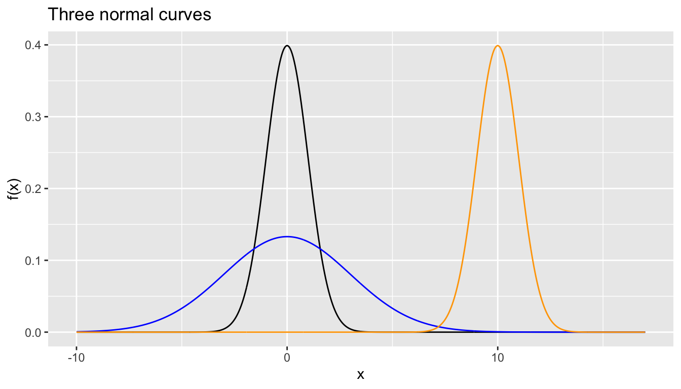
FIGURE A.1: Three examples of normal curves.

Some notes about these curves:

The black curve is a specific case of normal distribution called the standard normal AKA z-curve AKA z-distribution
The blue normal curve has the same center as the black curve, but more spread/variation.
The orange normal curve has a different center than the black curve, but same spread/variation.

In Figure A.2, we illustrate some useful “rules of thumb” of how values that form a normal curve distribute:

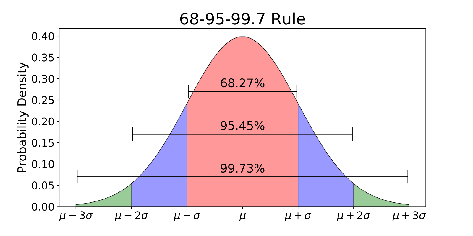
FIGURE A.2: Normal rules.

68.27% of values lie within \(\pm\) 1 standard deviation \(\sigma\) of mean \(\mu\) i.e. between \((\mu - \sigma, \mu + \sigma)\)
95.45% of values lie within \(\pm\) 2 standard deviations \(\sigma\) of mean \(\mu\) i.e. between \((\mu - 2\sigma, \mu + 2\sigma)\)
99.73% of values lie within \(\pm\) 3 standard deviations \(\sigma\) of mean \(\mu\) i.e. between \((\mu - 3\sigma, \mu + 3\sigma)\)

Some notes:

So about two-thirds of values that follow a bell-curve are within \(\pm\) 1 standard deviation \(\sigma\) of mean \(\mu\).
You might also see a similar statement of: 95% of values lie within \(\pm\) 1.96 standard deviations \(\sigma\) of mean \(\mu\)
Only 100% - 99.73% = 0.27% of values lie outside of the interval \((\mu - 3\sigma, \mu + 3\sigma)\). In other words, almost all values like within the interval that’s \(6\sigma\) lengths wide. This is where the term “six sigma” from manufacturing reliability originates.