Chapter 8 Sampling

In this chapter we kick off the third segment of this book, statistical inference, by learning about sampling. The concepts behind sampling form the basis of confidence intervals and hypothesis testing, which we’ll cover in Chapters 9 and 10 respectively. We will see that the tools that you learned in the data science segment of this book, in particular data visualization and data wrangling, will also play an important role here in the development of your understanding. As mentioned before, the concepts throughout this text all build into a culmination allowing you to “think with data.”

Needed packages

Let’s load all the packages needed for this chapter (this assumes you’ve already installed them). If needed, read Section 2.3 for information on how to install and load R packages.

library(dplyr)
library(ggplot2)
library(moderndive)

8.1 Sampling activity

Let’s start with a hands-on activity.

8.1.1 What proportion of this bowl’s balls are red?

Take a look at the bowl in Figure 8.1. It has a certain number of red and a certain number of white balls all of equal size. Furthermore, it appears the bowl has been mixed beforehand as there does not seem to be any particular pattern to the spatial distribution of red and white balls.

Let’s now ask ourselves, what proportion of this bowl’s balls are red?

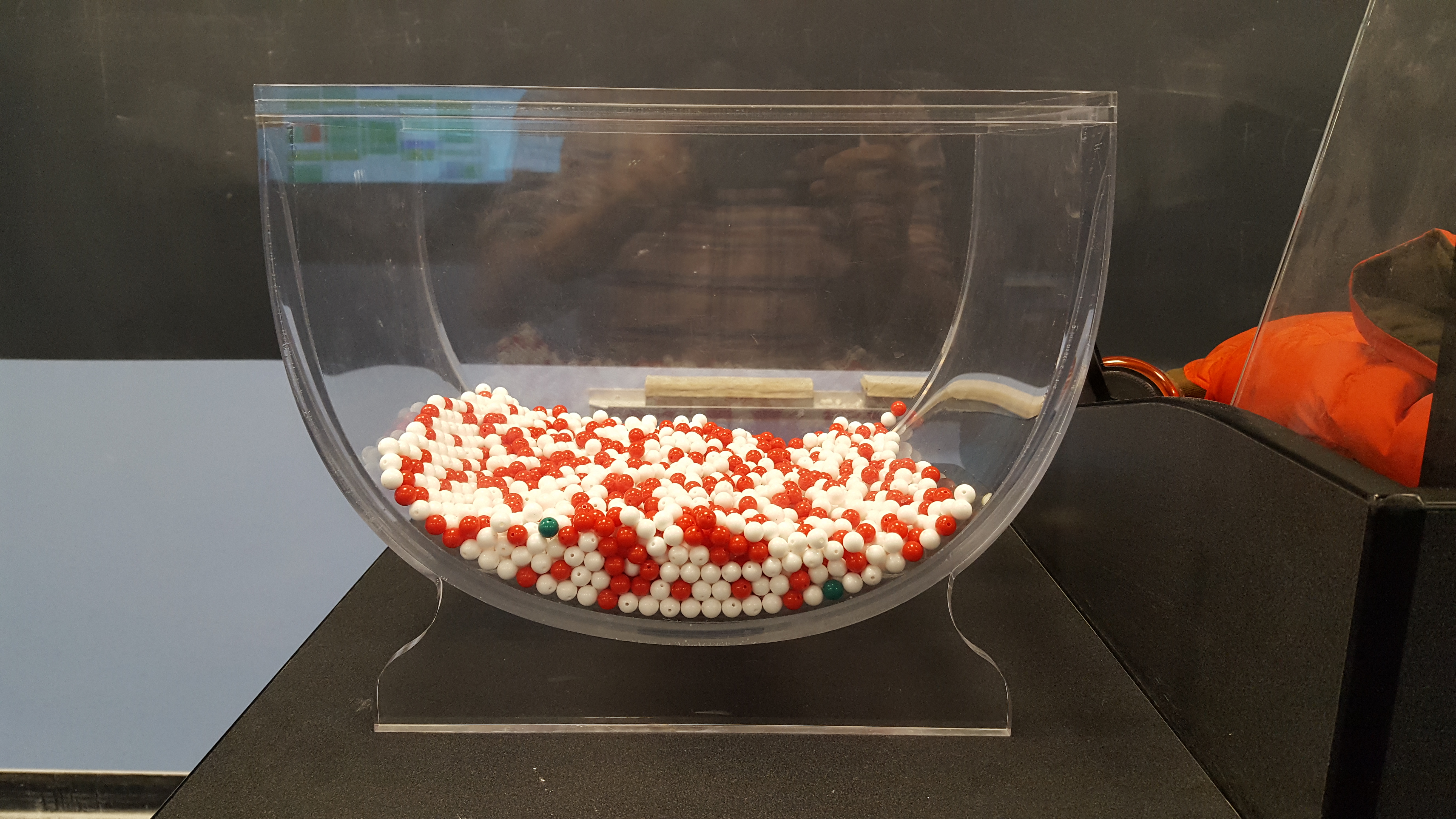
FIGURE 8.1: A bowl with red and white balls.

One way to answer this question would be to perform an exhaustive count: remove each ball individually, count the number of red balls and the number of white balls, and divide the number of red balls by the total number of balls. However this would be a long and tedious process.

8.1.2 Using the shovel once

Instead of performing an exhaustive count, let’s insert a shovel into the bowl as seen in Figure 8.2.

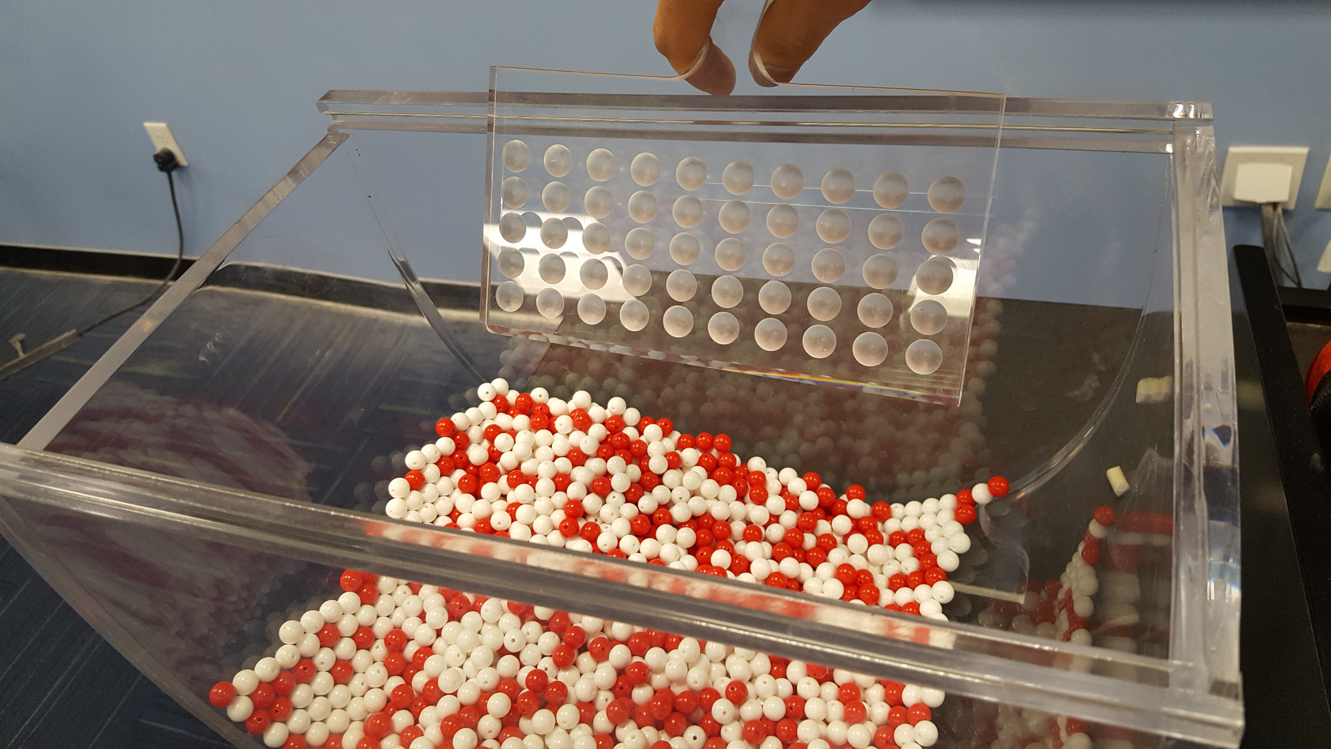
FIGURE 8.2: Inserting a shovel into the bowl.

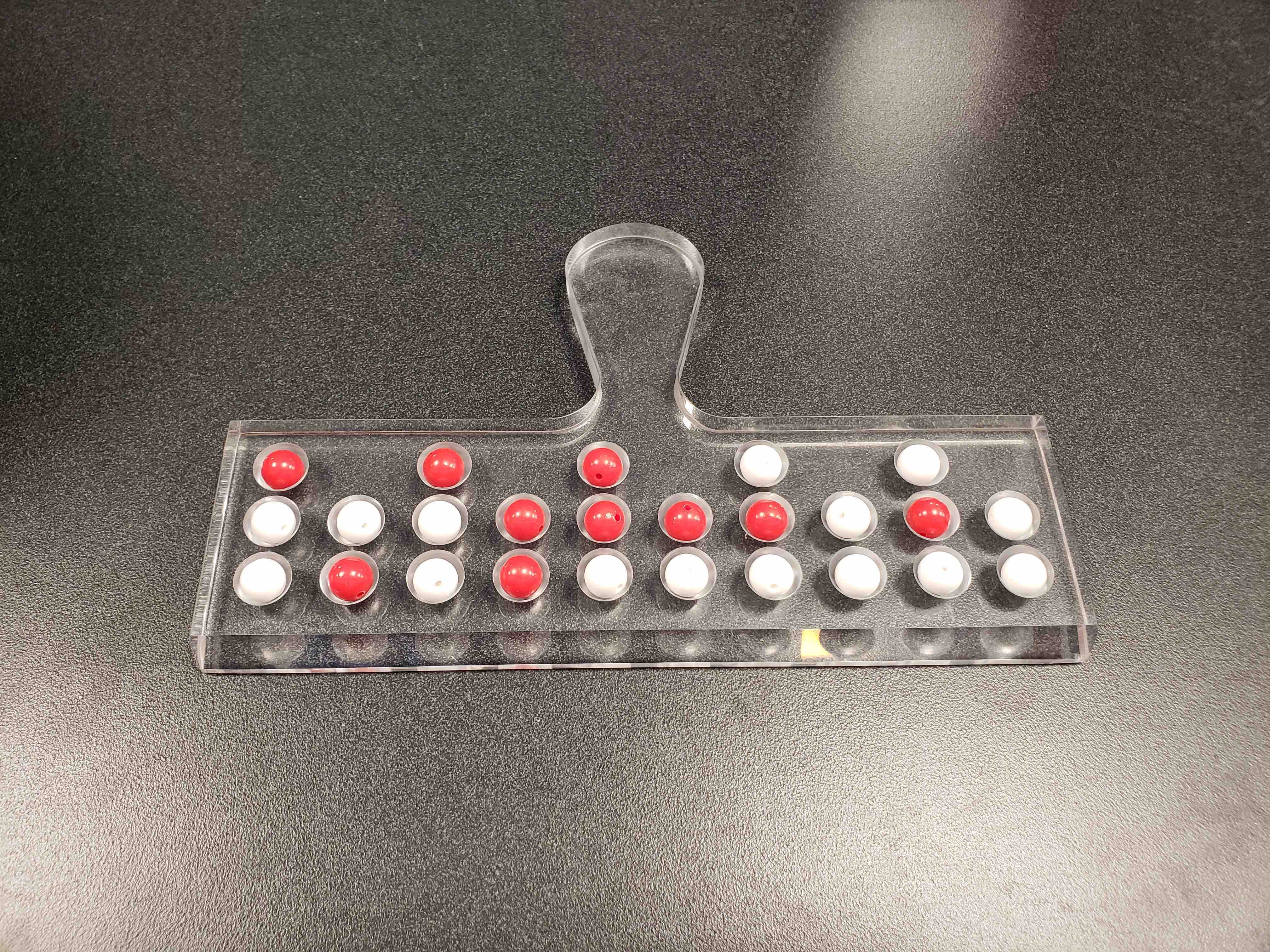
Using the shovel we remove a number of balls as seen in Figure 8.3.

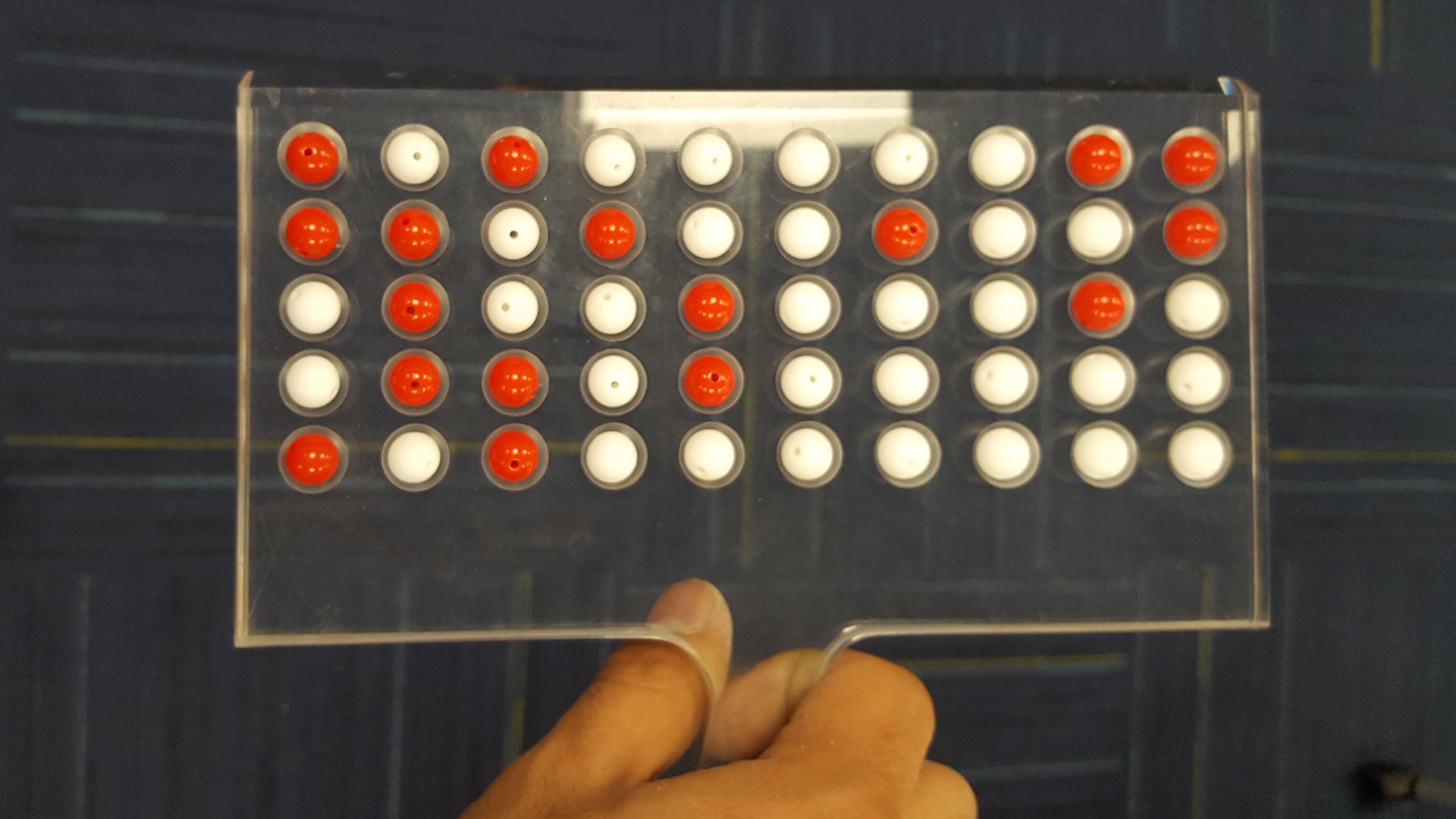
FIGURE 8.3: Fifty balls from the bowl.

Observe that 17 of the balls are red and there are a total of 5 x 10 = 50 balls and thus 0.34 = 34% of the shovel’s balls are red. We can view the proportion of balls that are red in this shovel as a guess of the proportion of balls that are red in the entire bowl. While not as exact as doing an exhaustive count, our guess of 34% took much less time and energy to obtain.

However, say, we started this activity over from the beginning. In other words, we replace the 50 balls back into the bowl and start over. Would we remove exactly 17 red balls again? In other words, would our guess at the proportion of the bowl’s balls that are red be exactly 34% again? Maybe?

What if we repeated this exercise several times? Would I obtain exactly 17 red balls each time? In other words, would our guess at the proportion of the bowl’s balls that are red be exactly 34% every time? Surely not. Let’s actually do and observe the results with the help of 33 of our friends.

8.1.3 Using the shovel 33 times

Each of our 33 friends will do the following:

use the shovel to remove 50 balls each,
count the number of red balls,
use this number to compute the proportion of the 50 balls they removed that are red,
return the balls into the bowl, and
mix the contents of the bowl a little to not let a previous group’s results influence the next group’s set of results.

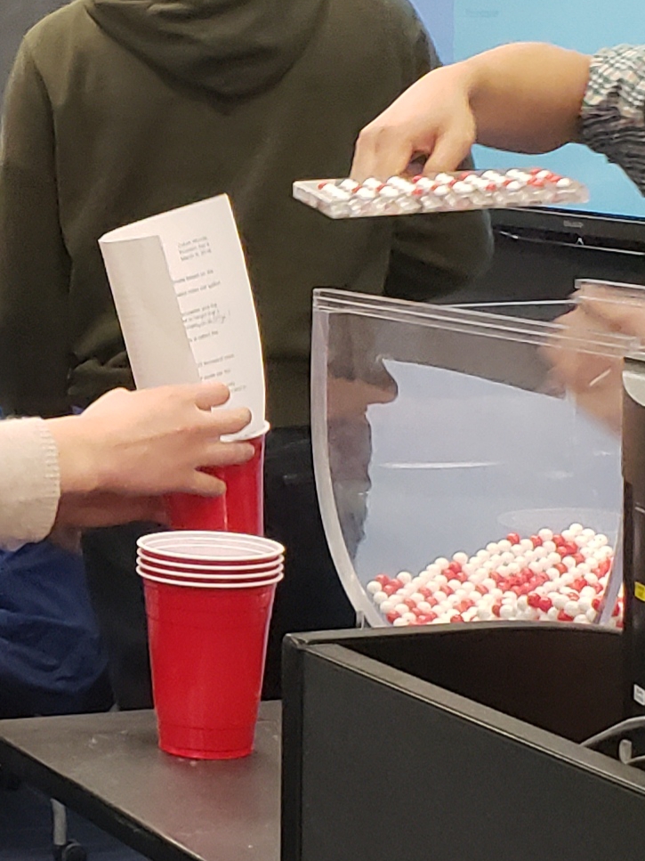
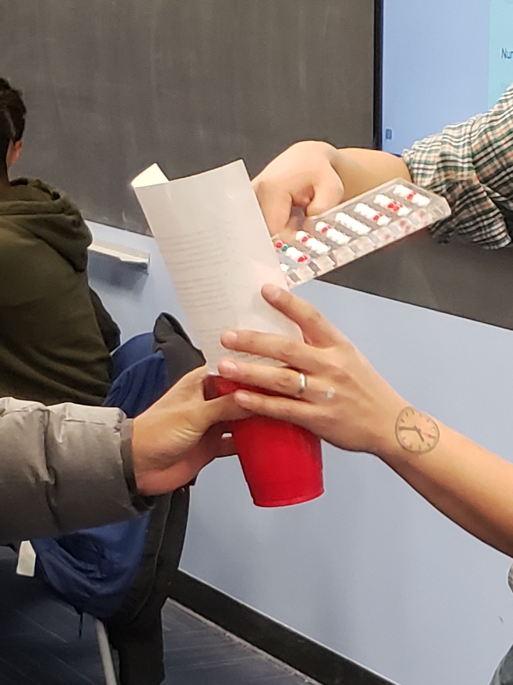
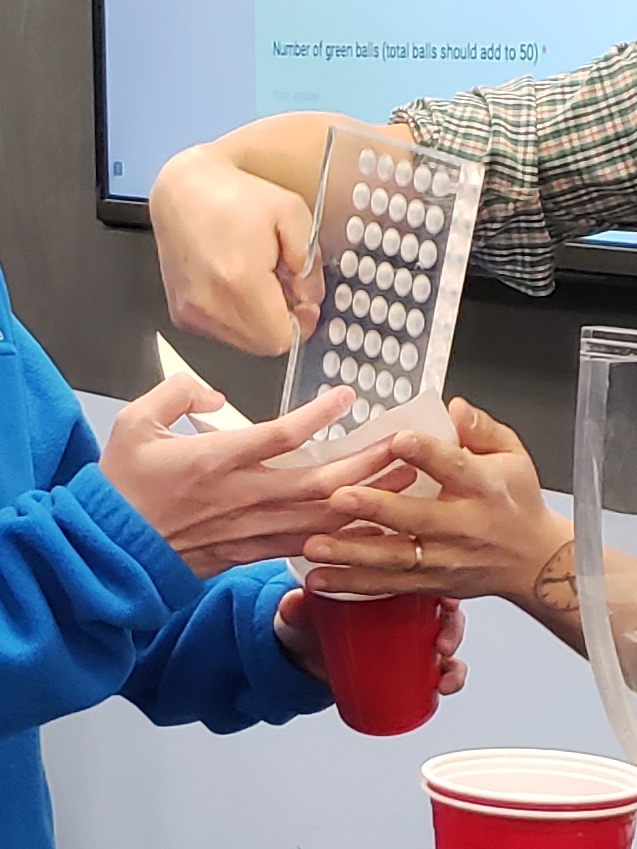
FIGURE 8.4: Repeating sampling activity 33 times.

However, before returning the balls into the bowl, they are going to mark the proportion of the 50 balls they removed that are red in a histogram as seen in Figure 8.5.

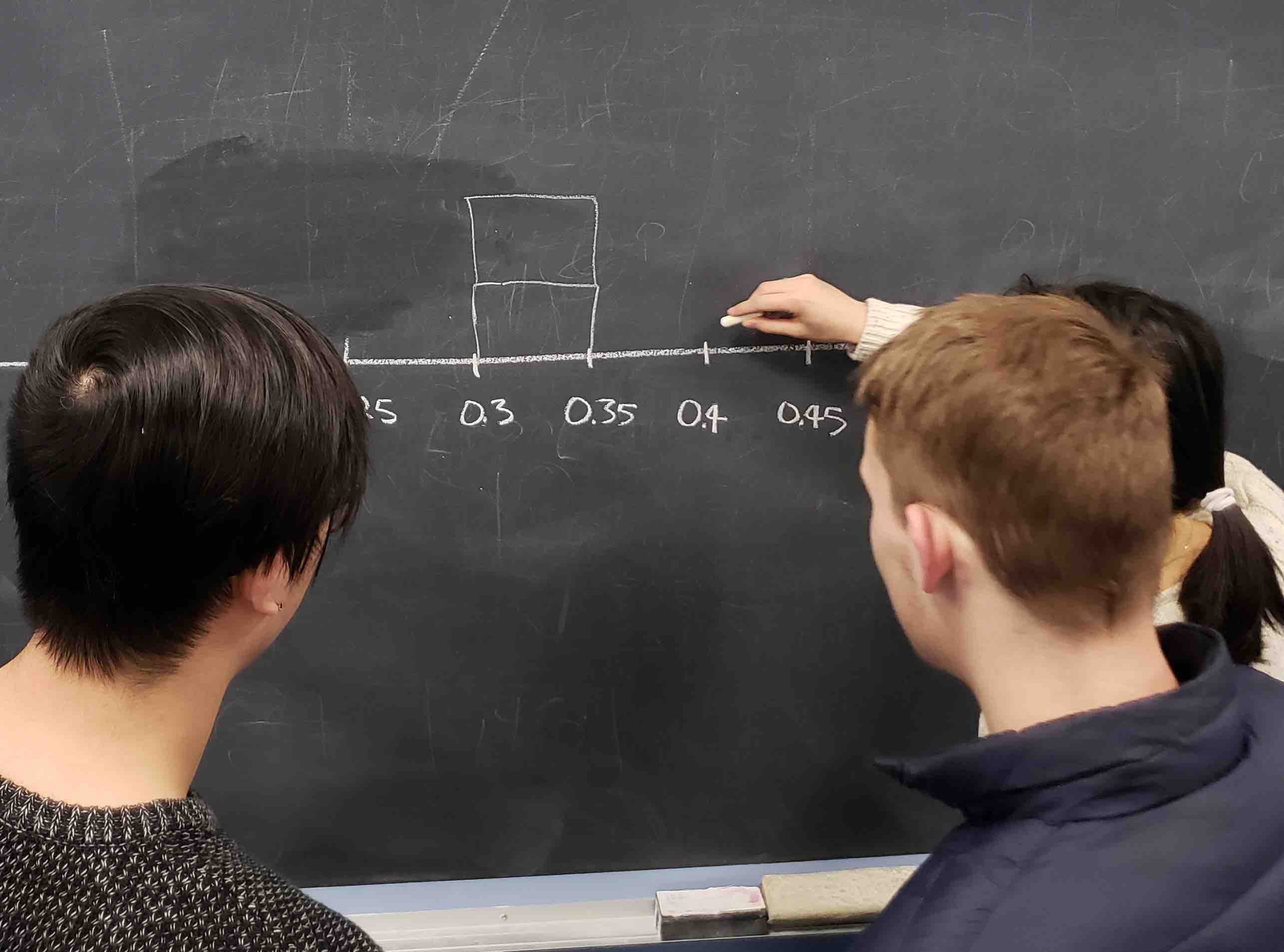
FIGURE 8.5: Constructing a histogram of proportions.

Recall from Section 3.5 that histograms allow us to visualize the distribution of a numerical variable: where the values center and in particular how they vary. The resulting hand-drawn histogram can be seen in Figure 8.6.

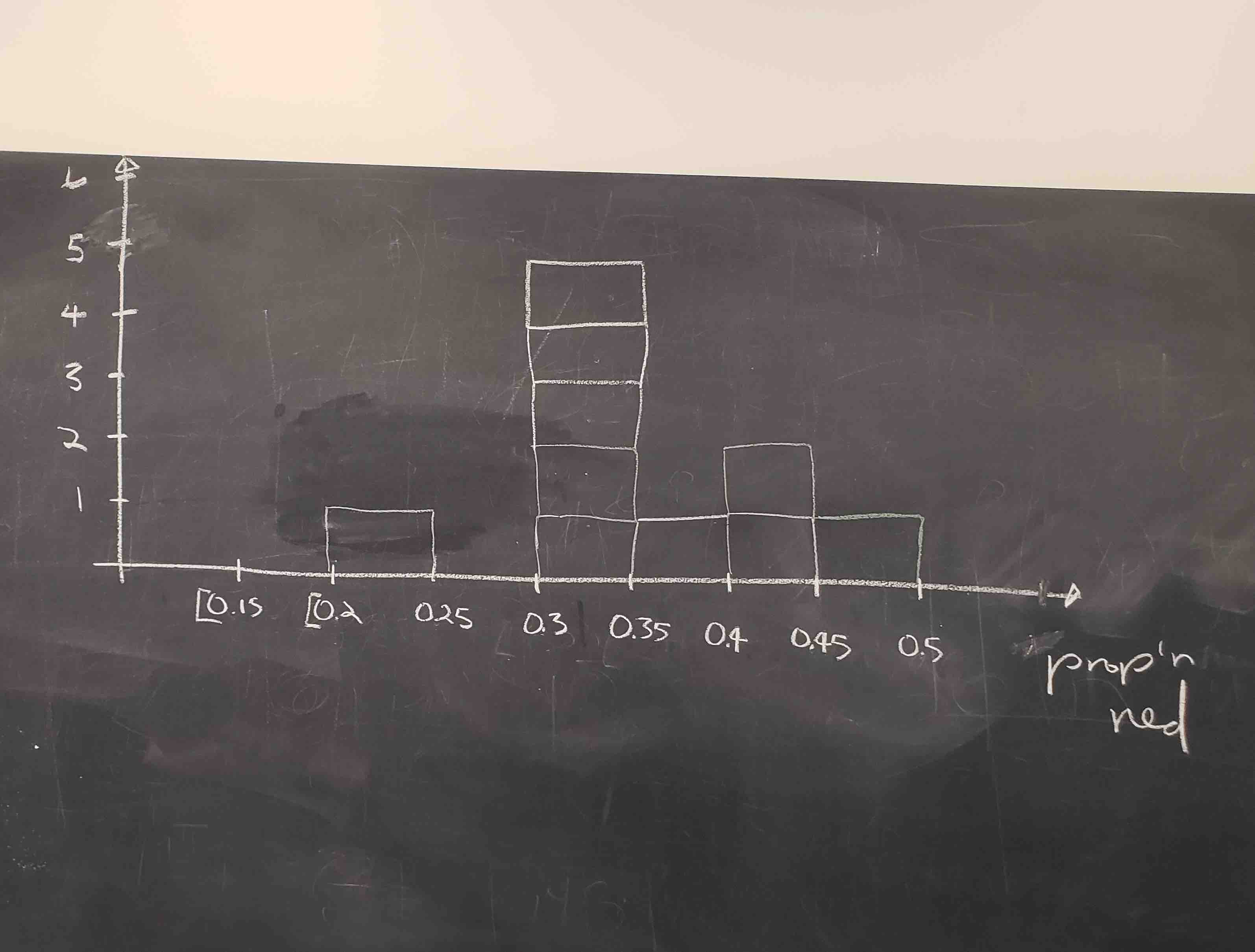
FIGURE 8.6: Hand-drawn histogram of 33 proportions.

Observe the following about the histogram in Figure 8.6:

At the low end, one group removed 50 balls from the bowl with proportion between 0.20 = 20% and 0.25 = 25%
At the high end, another group removed 50 balls from the bowl with proportion between 0.45 = 45% and 0.5 = 50% red.
However the most frequently occurring proportions were between 0.30 = 30% and 0.35 = 35% red, right in the middle of the distribution.
The shape of this distribution is somewhat bell-shaped.

Let’s construct this same hand-drawn histogram in R using your data visualization skills that you honed in Chapter 3. We saved our 33 group of friends’ proportion red in a data frame tactile_prop_red which is included in the moderndive package you loaded earlier.

tactile_prop_red
View(tactile_prop_red)

Let’s display only the first 10 out of 33 rows of tactile_prop_red’s contents in Table 8.1.

TABLE 8.1: First 10 out of 33 groups’ proportion of 50 balls that are red.
group	replicate	red_balls	prop_red
Ilyas, Yohan	1	21	0.42
Morgan, Terrance	2	17	0.34
Martin, Thomas	3	21	0.42
Clark, Frank	4	21	0.42
Riddhi, Karina	5	18	0.36
Andrew, Tyler	6	19	0.38
Julia	7	19	0.38
Rachel, Lauren	8	11	0.22
Daniel, Caroline	9	15	0.30
Josh, Maeve	10	17	0.34

Observe for each group we have their names, the number of red_balls they obtained, and the corresponding proportion out of 50 balls that were red named prop_red. Observe, we also have a variable replicate enumerating each of the 33 groups; we chose this name because each row can be viewed as one instance of a replicated activity: using the shovel to remove 50 balls and computing the proportion of those balls that are red.

We visualize the distribution of these 33 proportions using a geom_histogram() with binwidth = 0.05 in Figure 8.7, which is appropriate since the variable prop_red is numerical. This computer-generated histogram matches our hand-drawn histogram from the earlier Figure 8.6.

ggplot(tactile_prop_red, aes(x = prop_red)) +
  geom_histogram(binwidth = 0.05, boundary = 0.4, color = "white") +
  labs(x = "Proportion of 50 balls that were red", 
       title = "Distribution of 33 proportions red")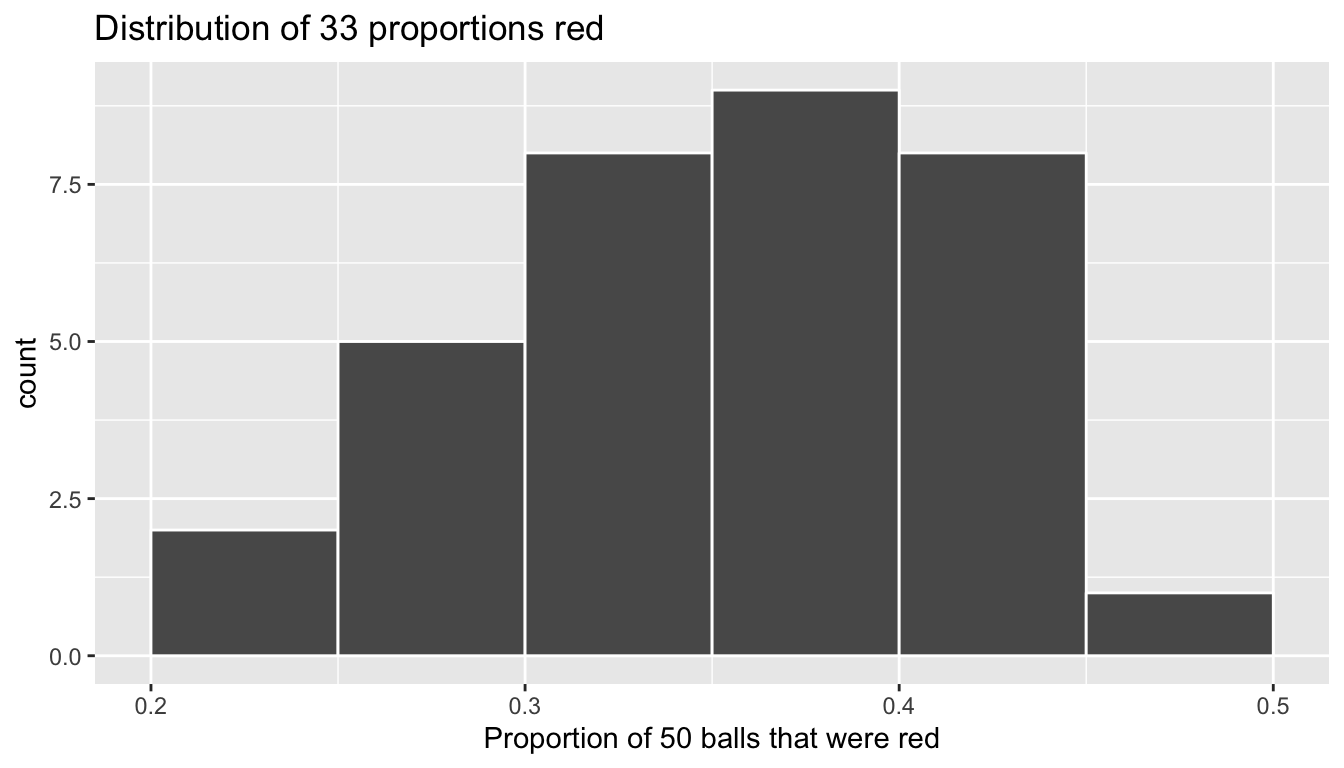

FIGURE 8.7: Distribution of 33 proportions based on 33 samples of size 50

8.1.4 What are we doing here?

What we just demonstrated in this activity is the statistical concept of sampling. We would like to know the proportion of the bowl’s balls that are red, but because the bowl has a very large number of balls performing an exhaustive count of the number of red and white balls in the bowl would be very costly in terms of both time and energy. We therefore extract a sample of 50 balls using the shovel. Using this sample of 50 balls, we estimate the proportion of the bowl’s balls that are red using the proportion of the shovel’s balls that are red. This estimate in our earlier example was 17 red balls out of 50 balls = 34%. Moreover, because we mixed the balls before each use of the shovel, the samples were randomly drawn. Because each sample was drawn at random, the samples were different from each other. Because the samples were different from each other, we obtained the different proportions red observed in Table 8.1. This is known as the concept of sampling variation.

In Section 8.2 we’ll mimic the hands-on sampling activity we just performed in a computer simulation; using a computer will allow us to repeat the above sampling activity much more than 33 times. Using a computer, not only will be able to repeat the hands-on activity a very large number of times, but we will also be able to repeat it using different sized shovels.

The purpose of these simulations is to develop an understanding of two key concepts relating to sampling: understanding the concept of sampling variation and the role that sample size plays in this variation. To this end, we’ll present you with definitions, terminology, and notation related to sampling in Section 8.3. As with many disciplines, there are definitions, terminology, and notation that seem very inaccessible and even confusing at first. However, as with many difficult topics, if you truly understand the underlying concepts and practice, practice, practice, you’ll be able to master these topics.

To tie the contents of this chapter to the real-word, we’ll present an example of one of the most recognizable uses of sampling: polls. In Section 8.4 we’ll look at a particular case study: a 2013 poll on then President Obama’s popularity among young Americans, conducted by the Harvard Kennedy School’s Institute of Politics.

We’ll close this chapter by generalizing the above sampling from the bowl activity to other scenarios, distinguishing between random sampling and random assignment, presenting the theoretical result underpinning all our results, and presenting a few mathematical formulas that relate to the concepts and ideas explored in this chapter.

8.2 Computer simulation

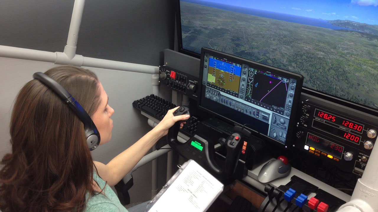
What we performed in Section 8.1 is a simulation of sampling. In other words, we were not in a real-life sampling scenario in order to answer a real-life question, but rather we were mimicking such a scenario with our bowl and shovel. The crowd-sourced Wikipedia definition of a simulation states: “A simulation is an approximate imitation of the operation of a process or system.”¹ One example of simulations in practice are a flight simulators: before pilots in training are allowed to fly an actual plane, they first practice on a computer that attempts to mimic the reality of flying an actual plane as best as possible.

Now you might be thinking that simulations must necessarily take place on computer. However, this is not necessarily true. Take for example crash test dummies: before cars are made available to the market, automobile engineers test their safety by mimicking the reality for passengers of being in an automobile crash. To distinguish between these two simulation types, we’ll term a simulation performed in real-life as a “tactile” simulation done with your hands and to the touch as opposed to a “virtual” simulation performed on a computer.

Example of a “tactile” simulation	Example of “virtual” simulation

So while in Section 8.1 we performed a “tactile” simulation of sampling using an actual bowl and an actual shovel with our hands, in this section we’ll perform a “virtual” simulation using a “virtual” bowl and a “virtual” shovel with our computers.

8.2.1 Using the virtual shovel once

Let’s start by performing the virtual analogue of the tactile sampling simulation we performed in 8.1. We first need a virtual analogue of the bowl seen in Figure 8.1. To this end, we included a data frame bowl in the moderndive package whose rows correspond exactly with the contents of the actual bowl.

bowl

# A tibble: 2,400 x 2
   ball_ID color
     <int> <chr>
 1       1 white
 2       2 white
 3       3 white
 4       4 red  
 5       5 white
 6       6 white
 7       7 red  
 8       8 white
 9       9 red  
10      10 white
# … with 2,390 more rows

Observe in the output that bowl has 2400 rows, telling us that the bowl contains 2400 equally-sized balls. The first variable ball_ID is used merely as an “identification variable” for this data frame as discussed in Subsection 2.4.4; none of the balls in the actual bowl are marked with numbers. The second variable color indicates whether a particular virtual ball is red or white. View the contents of the bowl in RStudio’s data viewer and scroll through the contents to convince yourselves that bowl is indeed a virtual version of the actual bowl in Figure 8.1.

Now that we have a virtual analogue of our bowl, we now need a virtual analogue for the shovel seen in Figure 8.2; we’ll use this virtual shovel to generate our virtual random samples of 50 balls. We’re going to use the rep_sample_n() function included in the moderndive package. This function allows us to take repeated, or replicated, samples of size n. Run the following and explore virtual_shovel’s contents in the RStudio viewer.

virtual_shovel <- bowl %>% 
  rep_sample_n(size = 50)
View(virtual_shovel)

Let’s display only the first 10 out of 50 rows of virtual_shovel’s contents in Table 8.2.

TABLE 8.2: First 10 sampled balls of 50 in virtual sample
replicate	ball_ID	color
1	1500	white
1	1767	red
1	1035	white
1	245	white
1	1121	white
1	1828	white
1	721	white
1	1729	red
1	770	white
1	1499	red

The ball_ID variable identifies which of the balls from bowl are included in our sample of 50 balls and color denotes its color. However what does the replicate variable indicate? In virtual_shovel’s case, replicate is equal to 1 for all 50 rows. This is telling us that these 50 rows correspond to a first repeated/replicated use of the shovel, in our case our first sample. We’ll see below when we “virtually” take 33 samples, replicate will take values between 1 and 33. Before we do this, let’s compute the proportion of balls in our virtual sample of size 50 that are red using the dplyr data wrangling verbs you learned in Chapter 4. Let’s breakdown the steps individually:

First, for each of our 50 sampled balls, identify if it is red using a test for equality using ==. For every row where color == "red", the Boolean TRUE is returned and for every row where color is not equal to "red", the Boolean FALSE is returned. Let’s create a new Boolean variable is_red using the mutate() function from Section 4.5:

virtual_shovel %>% 
  mutate(is_red = (color == "red"))

# A tibble: 50 x 4
# Groups:   replicate [1]
   replicate ball_ID color is_red
       <int>   <int> <chr> <lgl> 
 1         1    1500 white FALSE 
 2         1    1767 red   TRUE  
 3         1    1035 white FALSE 
 4         1     245 white FALSE 
 5         1    1121 white FALSE 
 6         1    1828 white FALSE 
 7         1     721 white FALSE 
 8         1    1729 red   TRUE  
 9         1     770 white FALSE 
10         1    1499 red   TRUE  
# … with 40 more rows

Second, we compute the number of balls out of 50 that are red using the summarize() function. Recall from Section 4.3 that summarize() takes a data frame with many rows and returns a data frame with a single row containing summary statistics that you specify, like mean() and median(). In this case we use the sum():

virtual_shovel %>% 
  mutate(is_red = (color == "red")) %>% 
  summarize(num_red = sum(is_red))

# A tibble: 1 x 2
  replicate num_red
      <int>   <int>
1         1      17

Why does this work? Because R treats TRUE like the number 1 and FALSE like the number 0. So summing the number of TRUE’s and FALSE’s is equivalent to summing 1’s and 0’s, which in the end counts the number of balls where color is red. In our case, 17 of the 50 balls were red.

Third and last, we compute the proportion of the 50 sampled balls that are red by dividing num_red by 50:

virtual_shovel %>% 
  mutate(is_red = color == "red") %>% 
  summarize(num_red = sum(is_red)) %>% 
  mutate(prop_red = num_red / 50)

# A tibble: 1 x 3
  replicate num_red prop_red
      <int>   <int>    <dbl>
1         1      17     0.34

In other words, this “virtual” sample’s balls were 34% red. Let’s make the above code a little more compact and succinct by combining the first mutate() and the summarize() as follows:

virtual_shovel %>% 
  summarize(num_red = sum(color == "red")) %>% 
  mutate(prop_red = num_red / 50)

# A tibble: 1 x 3
  replicate num_red prop_red
      <int>   <int>    <dbl>
1         1      17     0.34

Great! 34% of virtual_shovel’s 50 balls were red! So based on this particular sample, our guess at the proportion of the bowl’s balls that are red is 34%. But remember from our earlier tactile sampling activity that if we repeated this sampling, we would not necessarily obtain a sample of 50 balls with 34% of them being red again; there will likely be some variation. In fact in Table 8.2 we displayed 33 such proportions based on 33 tactile samples and then in Figure 8.6 we visualized the distribution of the 33 proportions in a histogram. Let’s now perform the virtual analogue of having 33 groups of students use the sampling shovel!

8.2.2 Using the virtual shovel 33 times

Recall that in our tactile sampling exercise in Section 8.1 we had 33 groups of students each use the shovel, yielding 33 samples of size 50 balls, which we then used to compute 33 proportions. In other words we repeated/replicated using the shovel 33 times. We can perform this repeated/replicated sampling virtually by once again using our virtual shovel function rep_sample_n(), but by adding the reps = 33 argument, indicating we want to repeat the sampling 33 times. Be sure to scroll through the contents of virtual_samples in RStudio’s viewer.

virtual_samples <- bowl %>% 
  rep_sample_n(size = 50, reps = 33)
View(virtual_samples)

Observe that while the first 50 rows of replicate are equal to 1, the next 50 rows of replicate are equal to 2. This is telling us that the first 50 rows correspond to the first sample of 50 balls while the next 50 correspond to the second sample of 50 balls. This pattern continues for all reps = 33 replicates and thus virtual_samples has 33 $\times$ 50 = 1650 rows.

Let’s now take the data frame virtual_samples with 33 $\times$ 50 = 1650 rows corresponding to 33 samples of size 50 balls and compute the resulting 33 proportions red. We’ll use the same dplyr verbs as we did in the previous section, but this time with an additional group_by() of the replicate variable. Recall from Section 4.4 that by assigning the grouping variable “meta-data” before summarizing(), we’ll obtain 33 different proportions red:

virtual_prop_red <- virtual_samples %>% 
  group_by(replicate) %>% 
  summarize(red = sum(color == "red")) %>% 
  mutate(prop_red = red / 50)
View(virtual_prop_red)

Let’s display only the first 10 out of 33 rows of virtual_prop_red’s contents in Table 8.1. As one would expect, there is variation in the resulting prop_red proportions red for the first 10 out 33 repeated/replicated samples.

TABLE 8.3: First 10 out of 33 virtual proportion of 50 balls that are red.
replicate	red	prop_red
1	18	0.36
2	20	0.40
3	19	0.38
4	18	0.36
5	15	0.30
6	18	0.36
7	19	0.38
8	13	0.26
9	23	0.46
10	14	0.28

Let’s visualize the distribution of these 33 proportions red based on 33 virtual samples using a histogram with binwidth = 0.05 in Figure 8.8.

ggplot(virtual_prop_red, aes(x = prop_red)) +
  geom_histogram(binwidth = 0.05, boundary = 0.4, color = "white") +
  labs(x = "Proportion of 50 balls that were red", 
       title = "Distribution of 33 proportions red")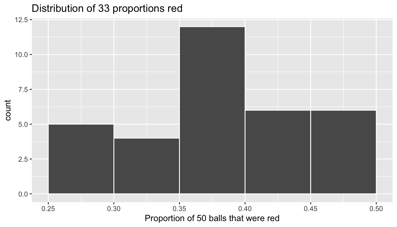

FIGURE 8.8: Distribution of 33 proportions based on 33 samples of size 50

Observe that occasionally we obtained proportions red that are less than 0.3 = 30%, while on the other hand we occasionally we obtained proportions that are greater than 0.45 = 45%. However, the most frequently occurring proportions red out of 50 balls were between 35% and 40% (for 11 out 33 samples). Why do we have these differences in proportions red? Because of sampling variation.

Let’s now compare our virtual results with our tactile results from the previous section in Figure 8.9. We see that both histograms, in other words the distribution of the 33 proportions red, are somewhat similar in their center and spread although not identical. These slight differences are again due to random variation. Furthermore both distributions are somewhat bell-shaped.

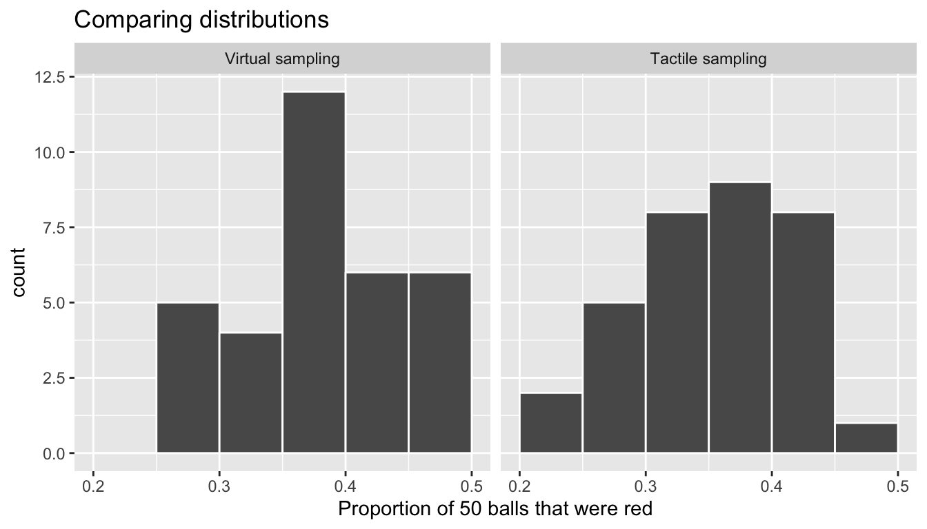
FIGURE 8.9: Comparing 33 virtual and 33 tactile proportions red.

8.2.3 Using the virtual shovel 1000 times

Now say we want study the variation in proportions red not based on 33 repeated/replicated samples, but rather a very large number of samples say 1000 samples. We have two choices at this point. We could have our students manually take 1000 samples of 50 balls and compute the corresponding 1000 proportion red out 50 balls. This would be cruel and unusual however, as this would be very tedious and time-consuming. This is where computers excel: automating long and repetitive tasks while performing them very quickly. Therefore at this point we will abandon tactile sampling in favor of only virtual sampling. Let’s once again use the rep_sample_n() function with sample size set to 50 once again, but this time with the number of replicates reps = 1000. Be sure to scroll through the contents of virtual_samples in RStudio’s viewer.

virtual_samples <- bowl %>% 
  rep_sample_n(size = 50, reps = 1000)
View(virtual_samples)

Observe that now virtual_samples has 1000 $\times$ 50 = 50,000 rows, instead of the 33 $\times$ 50 = 1650 rows from earlier. Using the same code as earlier, let’s take the data frame virtual_samples with 1000 $\times$ 50 = 50,000 and compute the resulting 1000 proportions red.

virtual_prop_red <- virtual_samples %>% 
  group_by(replicate) %>% 
  summarize(red = sum(color == "red")) %>% 
  mutate(prop_red = red / 50)
View(virtual_prop_red)

Observe that we now have 1000 replicates of prop_red, the proportion of 50 balls that are red. Using the same code as earlier, let’s now visualize the distribution of these 1000 replicates of prop_red in a histogram in Figure 8.10.

ggplot(virtual_prop_red, aes(x = prop_red)) +
  geom_histogram(binwidth = 0.05, boundary = 0.4, color = "white") +
  labs(x = "Proportion of 50 balls that were red", 
       title = "Distribution of 1000 proportions red")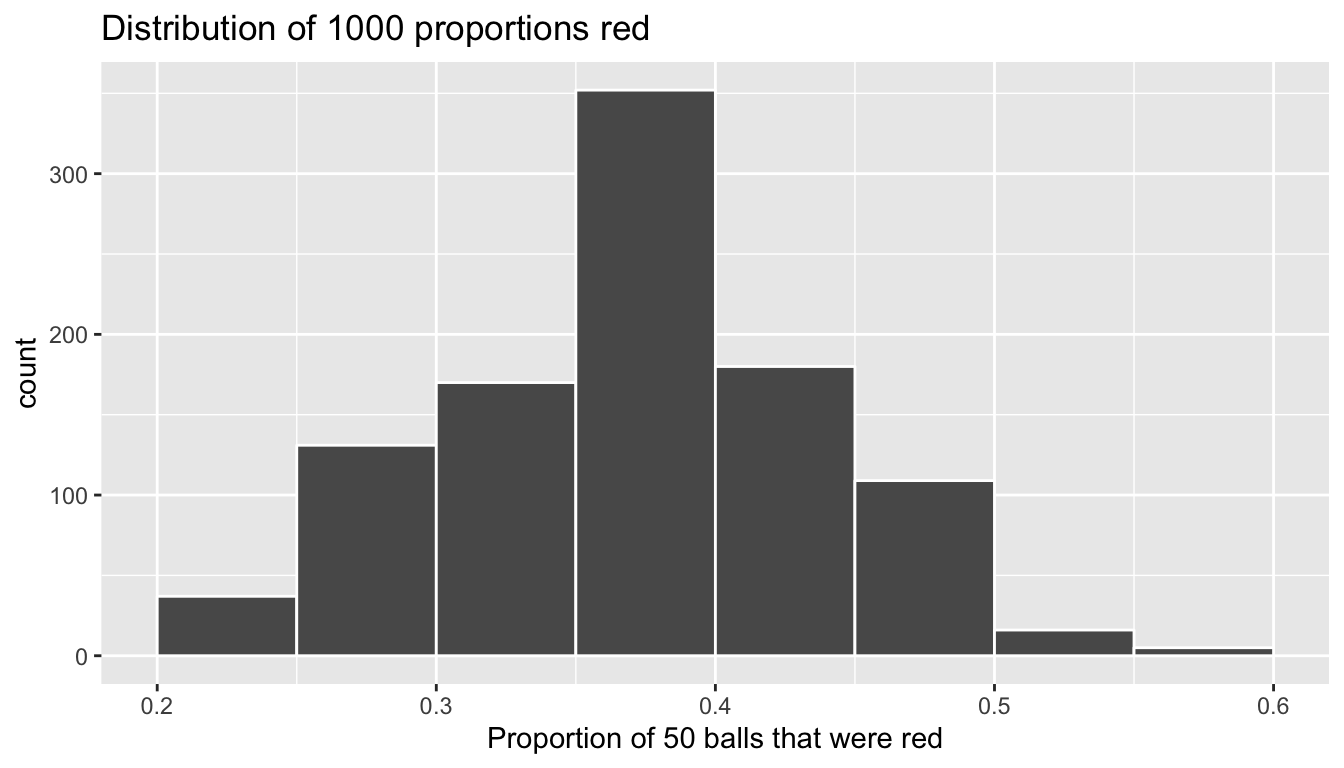

FIGURE 8.10: Distribution of 1000 proportions based on 33 samples of size 50

Once again, the most frequently occurring proportions red occur between 35% and 40%. Every now and then, we obtain proportions as low as between 20% and 25%, and others as high as between 55% and 60%. These are rare however. Furthermore observe that we now have a much more symmetric and smoother bell-shaped distribution. This distribution is in fact a Normal distribution; see Appendix A for a brief discussion on properties of the Normal distribution.

8.2.4 Using different shovels

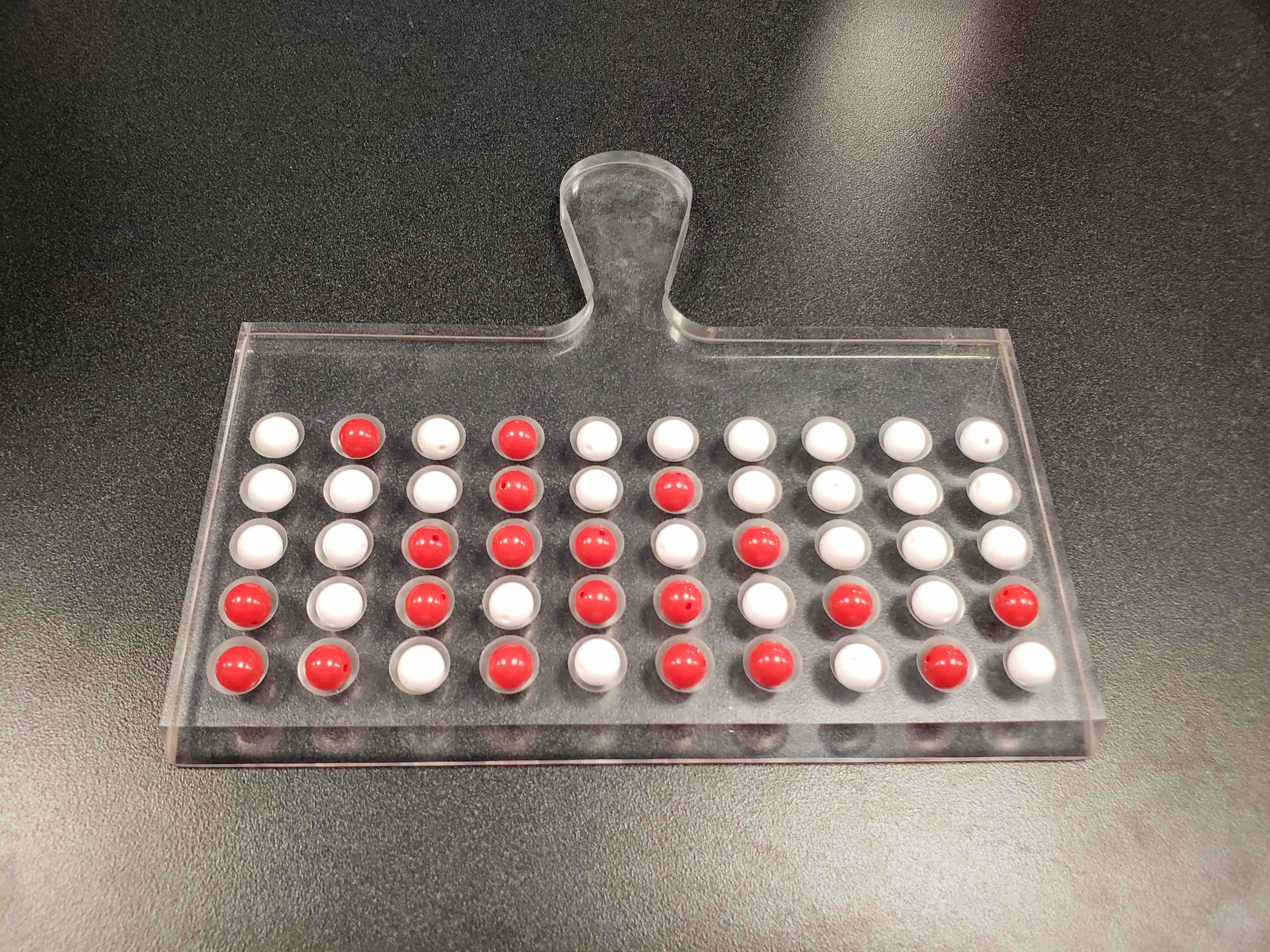
Now say instead of just one shovel, you had three choices of shovels to extract a sample of balls with.

A shovel with 25 slots	A shovel with 50 slots	A shovel with 100 slots

If your goal was still to estimate the proportion of the bowl’s balls that were red, which shovel would you choose? In our experience, most people would choose the shovel with 100 slots since it has the biggest sample size and hence would yield the “best” guess of the proportion of the bowl’s 2400 balls that are red. Using our newly developed tools for virtual sampling simulations, let’s unpack the effect of having different sample sizes! In other words, let’s use rep_sample_n() with size = 25, size = 50, and size = 100, while keeping the number of repeated/replicated samples at 1000:

Virtually use the appropriate shovel to generate 1000 samples with size balls.
Compute the resulting 1000 replicated of the proportion of the shovel’s balls that are red.
Visualize the distribution of these 1000 proportion red using a histogram.

Run each of the following code segments individually and then compare the three resulting histograms.

# Segment 1: sample size = 25 ------------------------------
# 1.a) Virtually use shovel 1000 times
virtual_samples_25 <- bowl %>% 
  rep_sample_n(size = 25, reps = 1000)

# 1.b) Compute resulting 1000 replicates of proportion red
virtual_prop_red_25 <- virtual_samples_25 %>% 
  group_by(replicate) %>% 
  summarize(red = sum(color == "red")) %>% 
  mutate(prop_red = red / 25)

# 1.c) Plot distribution via a histogram
ggplot(virtual_prop_red_25, aes(x = prop_red)) +
  geom_histogram(binwidth = 0.05, boundary = 0.4, color = "white") +
  labs(x = "Proportion of 25 balls that were red", title = "25") 

# Segment 2: sample size = 50 ------------------------------
# 2.a) Virtually use shovel 1000 times
virtual_samples_50 <- bowl %>% 
  rep_sample_n(size = 50, reps = 1000)

# 2.b) Compute resulting 1000 replicates of proportion red
virtual_prop_red_50 <- virtual_samples_50 %>% 
  group_by(replicate) %>% 
  summarize(red = sum(color == "red")) %>% 
  mutate(prop_red = red / 50)

# 2.c) Plot distribution via a histogram
ggplot(virtual_prop_red_50, aes(x = prop_red)) +
  geom_histogram(binwidth = 0.05, boundary = 0.4, color = "white") +
  labs(x = "Proportion of 50 balls that were red", title = "50")  

# Segment 3: sample size = 100 ------------------------------
# 3.a) Virtually using shovel with 100 slots 1000 times
virtual_samples_100 <- bowl %>% 
  rep_sample_n(size = 100, reps = 1000)

# 3.b) Compute resulting 1000 replicates of proportion red
virtual_prop_red_100 <- virtual_samples_100 %>% 
  group_by(replicate) %>% 
  summarize(red = sum(color == "red")) %>% 
  mutate(prop_red = red / 100)

# 3.c) Plot distribution via a histogram
ggplot(virtual_prop_red_100, aes(x = prop_red)) +
  geom_histogram(binwidth = 0.05, boundary = 0.4, color = "white") +
  labs(x = "Proportion of 100 balls that were red", title = "100")

For easy comparison, we present the three resulting histograms in a single row with matching x and y axes in Figure 8.11. What do you observe?

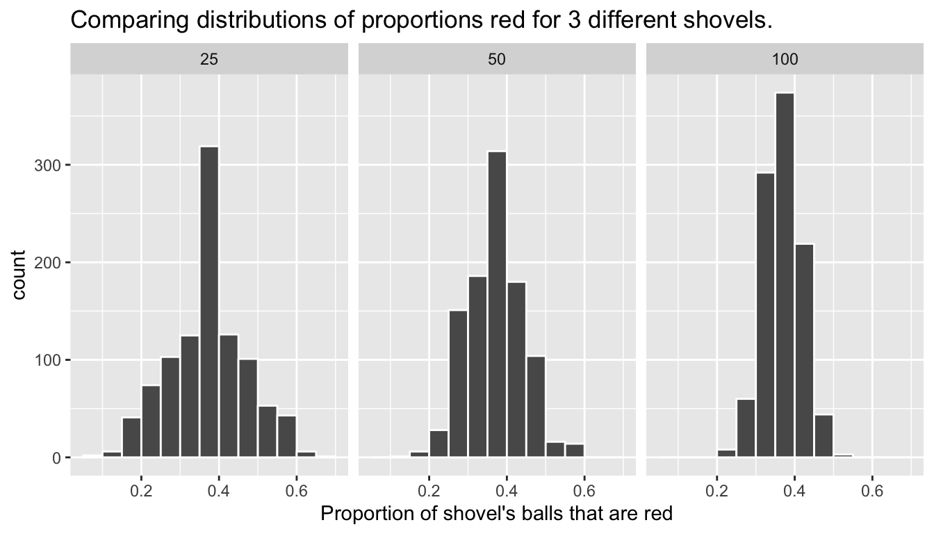
FIGURE 8.11: Comparing the distributions of proportion red for different sample sizes

Observe that as the sample size increases, the spread of the 1000 replicates of the proportion red decreases. In other words, as the sample size increases, there are less differences due to sampling variation and the distribution centers more tightly around the same value. Eyeballing Figure 8.11, things appear to center tightly around roughly 40%.

We can be numerically explicit about the amount of spread in our 3 sets of 1000 values of prop_red using the standard deviation: a summary statistic that measures the amount of spread and variation within a numerical variable; see Appendix A for a brief discussion on properties of the standard deviation. For all three sample sizes, let’s compute the standard deviation of the 1000 proportions red by running the following data wrangling code that uses the sd() summary function.

# n = 25
virtual_prop_red_25 %>% 
  summarize(sd = sd(prop_red))

# n = 50
virtual_prop_red_50 %>% 
  summarize(sd = sd(prop_red))

# n = 100
virtual_prop_red_100 %>% 
  summarize(sd = sd(prop_red))

Let’s compare these 3 measures of spread of the distributions in Table 8.4.

TABLE 8.4: Comparing standard deviations of proportions red for 3 different shovels.
Number of slots in shovel	Standard deviation of proportions red
25	0.099
50	0.071
100	0.048

As we observed visually in Figure 8.11, as the sample size increases our numerical measure of spread decreases; there is less variation in our proportions red. In other words, as the sample size increases, our guesses at the true proportion of the bowl’s balls that are red get more consistent and precise.

8.3 Sampling framework

In both our “hands-on” tactile simulations and our “virtual” simulations using a computer, we used sampling for the purpose of estimation: we extract samples in order to estimate the proportion of the bowl’s balls that are red. We used sampling as a cheaper and less-time consuming approach than to do a full census of all the balls. Our virtual simulations all built up to the results shown in Figure 8.11 and Table 8.4, comparing 1000 proportions red based on samples of size 25, 50, and 100. This was our first attempt at understanding two key concepts relating to sampling for estimation:

The effect of sampling variation on our estimates.
The effect of sample size on sampling variation.

Let’s now introduce some terminology and notation as well as statistical definitions related to sampling. Given the number of new words to learn, you will likely have to read these next three subsections multiple times. Keep in mind however that none of the concepts underlying these terminology, notation, and definitions are any different than the concepts underlying our simulations in Sections 8.1 and 8.2; it will simply take time and practice to master them.

8.3.1 Terminology & notation

Here is a list of terminology and mathematical notation relating to sampling. For each item, we’ll be sure to tie them to our simulations in Sections 8.1 and 8.2.

(Study) Population: A (study) population is a collection of individuals or observations about which we are interested. We mathematically denote the population’s size using upper case $N$. In our simulations the (study) population was the collection of $N$ = 2400 identically sized red and white balls contained in the bowl.
Population parameter: A population parameter is a numerical summary quantity about the population that is unknown, but you wish you knew. For example, when this quantity is a mean, the population parameter of interest is the population mean which is mathematically denoted with the Greek letter $\mu$ (pronounced “mu”). In our simulations however since we were interested in the proportion of the bowl’s balls that were red, the population parameter is the population proportion which is mathematically denoted with the letter $p$.
Census: An exhaustive enumeration or counting of all $N$ individuals or observations in the population in order to compute the population parameter’s value exactly. In our simulations, this would correspond to manually going over all $N$ = 2400 balls in the bowl and counting the number that are red and computing the population proportion $p$ of the balls that are red exactly. When the number $N$ of individuals or observations in our population is large, as was the case with our bowl, a census can be very expensive in terms of time, energy, and money.
Sampling: Sampling is the act of collecting a sample from the population when we don’t have the means to perform a census. We mathematically denote the sample’s size using lower case $n$, as opposed to upper case $N$ which denotes the population’s size. Typically the sample size $n$ is much smaller than the population size $N$, thereby making sampling a much cheaper procedure than a census. In our simulations, we used shovels with 25, 50, and 100 slots to extract a sample of size $n$ = 25, $n$ = 50, and $n$ = 100 balls.
Point estimate (AKA sample statistic): A summary statistic computed from the sample that estimates the unknown population parameter. In our simulations, recall that the unknown population parameter was the population proportion and that this is mathematically denoted with $p$. Our point estimate is the sample proportion: the proportion of the shovel’s balls that are red. In other words, it is our guess of the proportion of the bowl’s balls balls that are red. We mathematically denote the sample proportion using $\widehat{p}$; the “hat” on top of the $p$ indicates that it is an estimate of the unknown population proportion $p$.
Representative sampling: A sample is said be a representative sample if it is representative of the population. In other words, are the sample’s characteristics a good representation of the population’s characteristics? In our simulations, are the samples of $n$ balls extracted using our shovels representative of the bowl’s $N$=2400 balls?
Generalizability: We say a sample is generalizable if any results based on the sample can generalize to the population. In other words, can the value of the point estimate be generalized to estimate the value of the population parameter well? In our simulations, can we generalize the values of the sample proportions red of our shovels to the population proportion red of the bowl? Using mathematical notation, is $\widehat{p}$ a “good guess” of $p$?
Bias: In a statistical sense, we say bias occurs if certain individuals or observations in a population have a higher chance of being included in a sample than others. We say a sampling procedure is unbiased if every observation in a population had an equal chance of being sampled. In our simulations, since each ball had the same size and hence an equal chance of being sample in our shovels, our samples were unbiased.
Random sampling: We say a sampling procedure is random if we sample randomly from the population in an unbiased fashion. In our simulations, this would correspond to sufficiently mixing the bowl before each use of the shovel.

Phew, that’s a lot of new terminology and notation to learn! Let’s put them all together to describe the paradigm of sampling:

If the sampling of a sample of size $n$ is done at random, then

the sample is unbiased and representative of the population of size $N$, thus

any result based on the sample can generalize to the population, thus

the point estimate is a “good guess” of the unknown population parameter, thus

instead of performing a census, we can infer about the population using sampling.

Restricting consideration to a shovel with 50 slots from our simulations,

If we extract a sample of $n=50$ balls at random, in other words we mix the equally-sized balls before using the shovel, then

the contents of the shovel are an unbiased representation of the contents of the bowl’s 2400 balls, thus

any result based on the sample of balls can generalize to the bowl, thus

the sample proportion $\widehat{p}$ of the $n=50$ balls in the shovel that are red is a “good guess” of the population proportion $p$ of the $N$=2400 balls that are red, thus

instead of manually going over all the balls in the bowl, we can infer about the bowl using the shovel.

Note that last word we wrote in bold: infer. The act of “inferring” is to deduce or conclude (information) from evidence and reasoning. In our simulations, we wanted to infer about the proportion of the bowl’s balls that are red. Statistical inference is the theory, methods, and practice of forming judgments about the parameters of a population and the reliability of statistical relationships, typically on the basis of random sampling (Wikipedia). In other words, statistical inference is the act of inference via sampling. In the upcoming Chapter 9 on confidence intervals, we’ll introduce the infer package, which makes statistical inference “tidy” and transparent. It is why this third portion of the book is called “Statistical inference via infer”.

8.3.2 Statistical definitions

Now for some important statistical definitions related to sampling. As a refresher of our 1000 repeated/replicated virtual samples of size $n$ = 25, $n$ = 50, and $n$ = 100 in Section 8.2, let’s display Figure 8.11 again below.

These types of distributions have a special name: sampling distributions; their visualization displays the effect of sampling variation on the distribution of any point estimate, in this case the sample proportion $\widehat{p}$. Using these sampling distributions, for a given sample size $n$, we can make statements about what values we can typically expect. For example, observe the centers of all three sampling distributions: they are all roughly centered around 0.4 = 40%. Furthermore, observe that while we are somewhat likely to observe sample proportions red of 0.2 = 20% when using the shovel with 25 slots, we will almost never observe this sample proportion when using the shovel with 100 slots. Observe also the effect of sample size on the sampling variation. As the sample size $n$ increases from 25 to 50 to 100, the spread/variation of the sampling distribution decreases and thus the values cluster more and more tightly around the same center of around 40%. We quantified this spread/variation using the standard deviation of our proportions in Table 8.4, which we display again below:

Number of slots in shovel	Standard deviation of proportions red
25	0.099
50	0.071
100	0.048

So as the number of slots in the shovel increased, this standard deviation decreased. These types of standard deviations have another special name: standard errors; they quantify the effect of sampling variation induced on our estimates. In other words, they are quantifying how much we can expect different proportions of a shovel’s balls that are red to vary from random sample to random sample.

Unfortunately, many new statistics practitioners get confused by these names. For example, it’s common for people new to statistical inference to call the “sampling distribution” the “sample distribution”. Another additional source of confusion is the name “standard deviation” and “standard error”. Remember that a standard error is merely a kind of standard deviation: the standard deviation of any point estimate from a sampling scenario. In other words, all standard errors are standard deviations, but not all standard deviations are a standard error.

To help reinforce these concepts, let’s re-display Figure 8.11 but using our new terminology, notation, and definitions relating to sampling in Figure 8.12.

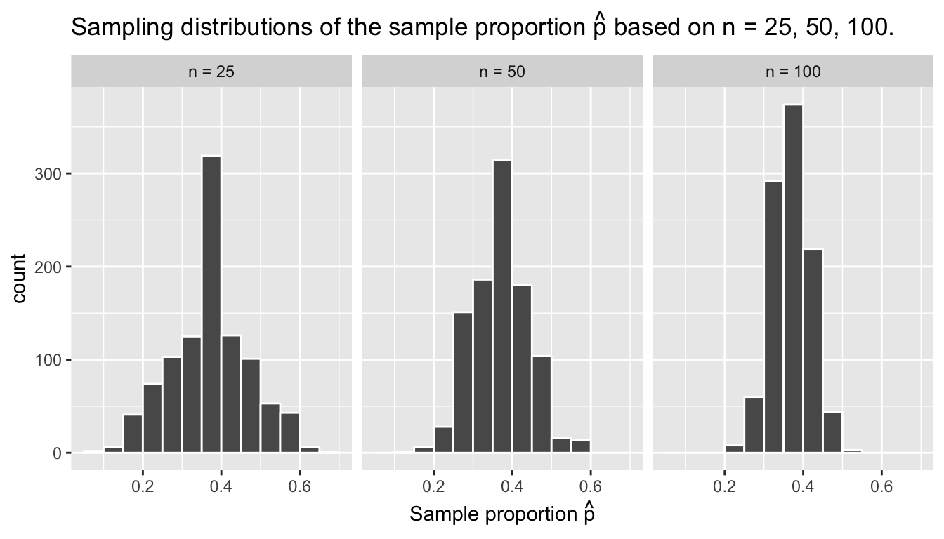
$Three sampling distributions of the sample proportion $\widehat{p}$.$

FIGURE 8.12: Three sampling distributions of the sample proportion $\widehat{p}$.

Furthermore, let’s re-display Table 8.4 but using our new terminology, notation, and definitions relating to sampling in Table 8.5.

TABLE 8.5: Three standard errors of the sample proportion $\widehat{p}$ based on n = 25, 50, 100.
Sample size	Standard error of $\widehat{p}$
n = 25	0.099
n = 50	0.071
n = 100	0.048

Remember the key message of this last table: that as the sample size $n$ goes up, the “typical” error of your point estimate as quantified by the standard error will go down.

8.3.3 The moral of the story

Let’s recap this section so far. We’ve seen that if a sample is generated at random, then the resulting point estimate is a “good guess” of the true unknown population parameter. In our simulations, since we made sure to mix the balls first before extracting a sample with the shovel, the resulting sample proportion $\widehat{p}$ of the shovel’s balls that were red was a “good guess” of the population proportion $p$ of the bowl’s balls that were red.

However, what do we mean by our point estimate being a “good guess”? While sometimes we’ll obtain a point estimate less than the true value of the unknown population parameter, other times we’ll obtain a point estimate greater than the true value of the unknown population parameter, this is because of sampling variation. However despite this sampling variation, our point estimates will “on average” be correct. In our simulations, sometimes our sample proportion $\widehat{p}$ was less than the true population proportion $p$, other times the sample proportion $\widehat{p}$ was greater than the true population proportion $p$. This was due to the sampling variability induced by the mixing. However despite this sampling variation, our sample proportions $\widehat{p}$ were always centered around the true population proportion. This is also known as having an accurate estimate.

What was the value of the population proportion $p$ of the $N$ = 2400 balls in the actual bowl? There were 900 red balls, for a proportion red of 900/2400 = 0.375 = 37.5%! How do we know this? Did the authors do an exhaustive count of all the balls? No! They were listed on the contexts of the box that the bowl came in. Hence we made the contents of the virtual bowl match the tactile bowl:

bowl %>% 
  summarize(sum_red = sum(color == "red"), 
            sum_not_red = sum(color != "red"))

# A tibble: 1 x 2
  sum_red sum_not_red
    <int>       <int>
1     900        1500

Let’s re-display our sampling distributions from Figures 8.11 and 8.12, but now with a vertical red line marking the true population proportion $p$ of balls that are red = 37.5% in Figure 8.13. We see that while there is a certain amount of error in the sample proportions $\widehat{p}$ for all three sampling distributions, on average the $\widehat{p}$ are centered at the true population proportion red $p$.

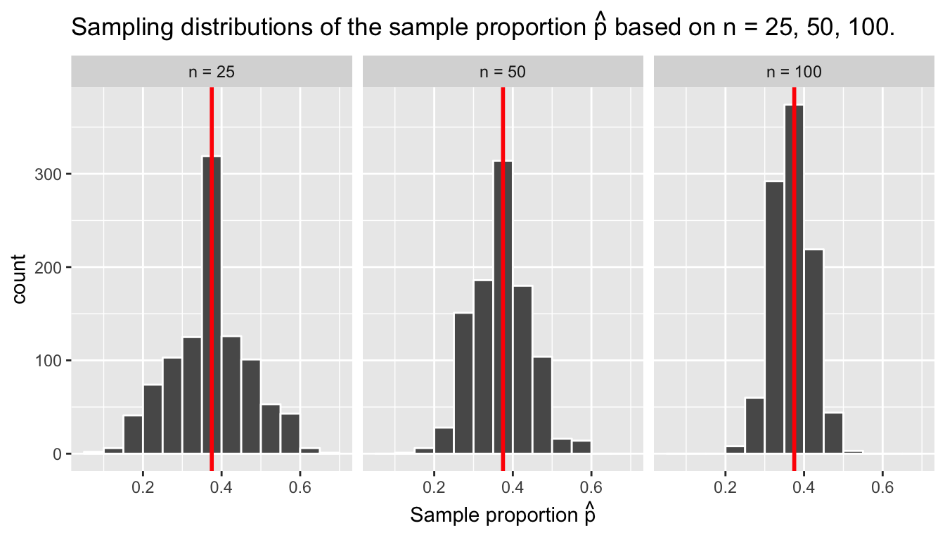
FIGURE 8.13: Three sampling distributions with population proportion $p$ marked in red.

We also saw in this section that as your sample size $n$ increases, your point estimates will vary less and less and be more and more concentrated around the true population parameter; this is quantified by the decreasing standard error. In other words, the typical error of your point estimates will decrease. In our simulations, as the sample size increases, the spread/variation of our sample proportions $\widehat{p}$ around the true population proportion $p$ decreases. You can observe this behavior as well in Figure 8.13. This is also known as having a more precise estimate.

So random sampling ensures our point estimates are accurate, while having a large sample size ensures our point estimates are precise. While accuracy and precision may sound like the same concept, they are actually not. Accuracy relates to how “on target” our estimates are whereas precision relates to how “consistent” our estimates are. Figure 8.14 illustrates the difference.

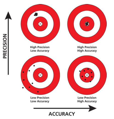
FIGURE 8.14: Comparing accuracy and precision

As this point you might be asking yourself: “If you already knew the true proportion of the bowl’s balls that are red was 37.5%, then what did we do any of this for?” In other words, “If you already knew the value of the true unknown population parameter, then why did we do any sampling?” You might also be asking: “Why did we take 1000 repeated/replicated samples of size n = 25, 50, and 100? Shouldn’t we be taking only one sample that’s as large as possible?” Recall our definition of a simulation from Section 8.2: an approximate imitation of the operation of a process or system. We performed these simulations to study:

The effect of sampling variation on our estimates.
The effect of sample size on sampling variation.

In a real-life scenario, we won’t know what the true value of the population parameter is and furthermore we won’t take repeated/replicated samples but rather a single sample that’s as large as we can afford. This was also done to show the power of the technique of sampling when trying to estimate a population parameter. Since we knew the value was 37.5%, we could show just how well the different sample sizes approximated this value in their sampling distributions. We present one case study of a real-life sampling scenario in the next section: polling.

8.4 Case study: Polls

In December 4, 2013 National Public Radio in the US reported on a recent, at the time, poll of President Obama’s approval rating among young Americans aged 18-29 in an article Poll: Support For Obama Among Young Americans Eroding. A quote from the article:

After voting for him in large numbers in 2008 and 2012, young Americans are souring on President Obama.

According to a new Harvard University Institute of Politics poll, just 41 percent of millennials — adults ages 18-29 — approve of Obama’s job performance, his lowest-ever standing among the group and an 11-point drop from April.

Let’s tie elements of the real-life poll in this new article with our “tactile” and “virtual” simulations from Sections 8.1 and 8.2 using the terminology, notations, and definitions we learned in Section 8.3.

(Study) Population: Who is the population of $N$ individuals or observations of interest?
- Simulation: $N$ = 2400 identically-sized red and white balls
- Obama poll: $N$ = ? young Americans aged 18-29
Population parameter: What is the population parameter?
- Simulation: The population proportion $p$ of ALL the balls in the bowl that are red.
- Obama poll: The population proportion $p$ of ALL young Americans who approve of Obama’s job performance.
Census: What would a census look like?
- Simulation: Manually going over all $N$ = 2400 balls and exactly computing the population proportion $p$ of the balls that are red, a time consuming task.
- Obama poll: Locating all $N$ = ? young Americans and asking them all if they approve of Obama’s job performance, an expensive task.
Sampling: How do you collect the sample of size $n$ individuals or observations?
- Simulation: Using a shovel with $n$ slots.
- Obama poll: One method is to get a list of phone numbers of all young Americans and pick out $n$ phone numbers. In this poll’s case, the sample size of this poll was $n$ = 2089 young Americans.
Point estimate (AKA sample statistic): What is your estimate of the unknown population parameter?
- Simulation: The sample proportion $\widehat{p}$ of the balls in the shovel that were red.
- Obama poll: The sample proportion $\widehat{p}$ of young Americans in the sample that approve of Obama’s job performance. In this poll’s case, $\widehat{p}$ = 0.41 = 41%, the quoted percentage in the second paragraph of the article.
Representative sampling: Is the sampling procedure representative?
- Simulation: Are the contents of the shovel representative of the contents of the bowl?
- Obama poll: Is the sample of $n$ = 2089 young Americans representative of all young Americans aged 18-29?
Generalizability: Are the samples generalizable to the greater population?
- Simulation: Is the sample proportion $\widehat{p}$ of the shovel’s balls that are red a “good guess” of the population proportion $p$ of the bowl’s balls that are red?
- Obama poll: Is the sample proportion $\widehat{p}$ = 0.41 of the sample of young Americans who support Obama a “good guess” of the population proportion $p$ of all young Americans who support Obama? In other words, can we confidently say that 41% of all young Americans approve of Obama?
Bias: Is the sampling procedure unbiased? In other words, do all observations have an equal chance of being included in the sample?
- Simulation: Since each ball was equally sized, each ball had an equal chance of being included in a shovel’s sample, and hence the sampling was unbiased.
- Obama poll: Did all young Americans have an equal chance at being represented in this poll? For example, if this was conducted using only mobile phone numbers, would people without mobile phones be included? What if those who disapproved of Obama were less likely to agree to take part in the poll? What about if this were an internet poll on a certain news website? Would non-readers of this website be included? We need to ask the Harvard University Institute of Politics pollsters about their sampling methodology.
Random sampling: Was the sampling random?
- Simulation: As long as you mixed the bowl sufficiently before sampling, your samples would be random.
- Obama poll: Was the sample conducted at random? We need to ask the Harvard University Institute of Politics pollsters about their sampling methodology.

Once again, let’s revisit the sampling paradigm:

If the sampling of a sample of size $n$ is done at random, then

the sample is unbiased and representative of the population of size $N$, thus

any result based on the sample can generalize to the population, thus

the point estimate is a “good guess” of the unknown population parameter, thus

instead of performing a census, we can infer about the population using sampling.

In our simulations using the shovel with 50 slots:

If we extract a sample of $n$ = 50 balls at random, in other words we mix the equally-sized balls before using the shovel, then

the contents of the shovel are an unbiased representation of the contents of the bowl’s 2400 balls, thus

any result based on the sample of balls can generalize to the bowl, thus

the sample proportion $\widehat{p}$ of the $n$ = 50 balls in the shovel that are red is a “good guess” of the population proportion $p$ of the $N$ = 2400 balls that are red, thus

instead of manually going over all the balls in the bowl, we can infer about the bowl using the shovel.

In the in-real life Obama poll:

If we had a way of contacting a randomly chosen sample of 2089 young Americans and poll their approval of Obama, then

these 2089 young Americans would be an unbiased and representative sample of all young Americans, thus

any results based on this sample of 2089 young Americans can generalize to the entire population of all young Americans, thus

the reported sample approval rating of 41% of these 2089 young Americans is a good guess of the true approval rating among all young Americans, thus

instead of performing a highly costly census of all young Americans, we can infer about all young Americans using polling.

8.5 Conclusion

8.5.1 Central Limit Theorem

What you did in Sections 8.1 and 8.2 (in particular in Figure 8.11 and Table 8.4) was demonstrate a very famous theorem, or mathematically proven truth, called the Central Limit Theorem. It loosely states that when sample means and sample proportions are based on larger and larger sample sizes, the sampling distribution of these two point estimates become more and more normally shaped and more and more narrow. In other words, their sampling distributions become more normally distributed and the spread/variation of these sampling distributions as quantified by their standard errors gets smaller. Shuyi Chiou, Casey Dunn, and Pathikrit Bhattacharyya created the following 3m38s video at https://www.youtube.com/embed/jvoxEYmQHNM explaining this crucial statistical theorem using the average weight of wild bunny rabbits and the average wing span of dragons as examples. Enjoy!

8.5.2 Summary table

In this chapter, we performed both tactile and virtual simulations of sampling to infer about an unknown proportion. We also presented a case study of a sampling in real life situation: polls. In both cases, we used the sample proportion $\widehat{p}$ to estimate the population proportion $p$. However, we are not just limited to scenarios related statistical inference for proportions. In other words, we can consider other population parameter and point estimate scenarios than just the population proportion $p$ and sample proportion $\widehat{p}$ scenarios we studied in this chapter. We present 5 more such scenarios in Table 8.6.

Note that the sample mean is traditionally noted as $\overline{x}$ but can also be thought of as an estimate of the population mean $\mu$. Thus, it can also be denoted as $\widehat{\mu}$ as shown below in the table.

TABLE 8.6: Scenarios of sampling for inference
Scenario	Population parameter	Notation	Point estimate	Notation.
1	Population proportion	$p$	Sample proportion	$\widehat{p}$
2	Population mean	$\mu$	Sample mean	$\widehat{\mu}$ or $\overline{x}$
3	Difference in population proportions	$p_1 - p_2$	Difference in sample proportions	$\widehat{p}_1 - \widehat{p}_2$
4	Difference in population means	$\mu_1 - \mu_2$	Difference in sample means	$\overline{x}_1 - \overline{x}_2$
5	Population regression slope	$\beta_1$	Sample regression slope	$\widehat{\beta}_1$ or $b_1$
6	Population regression intercept	$\beta_0$	Sample regression intercept	$\widehat{\beta}_0$ or $b_0$

We’ll cover all the remaining scenarios as follows, using the terminology, notation, and definitions related to sampling you saw in Section 8.3:

In Chapter 9, we’ll cover examples of statistical inference for
- Scenario 2: The mean age $\mu$ of all pennies in circulation in the US.
- Scenario 3: The difference $p_1 - p_2$ in the proportion of people who yawn when seeing someone else yawn and the proportion of people who yawn without seeing someone else yawn. This is an example of two-sample inference.
In Chapter 10, we’ll cover an example of statistical inference for
- Scenario 4: The difference $\mu_1 - \mu_2$ in average IMDB ratings for action and romance movies. This is another example of two-sample inference.
In Chapter 11, we’ll cover an example of statistical inference for the relationship between teaching score and various instructor demographic variables you saw in Chapter 6 on basic regression and Chapter 7 on multiple regression. Specifically
- Scenario 5: The intercept $\beta_0$ of some population regression line.
- Scenario 6: The slope $\beta_1$ of some population regression line.

8.5.3 Additional resources

An R script file of all R code used in this chapter is available here.

8.5.4 What’s to come?

Recall in our Obama poll case study in Section 8.4 that based on this particular sample, the Harvard University Institute of Politics’ best guess of Obama’s approval rating among all young Americans was 41%. However, this isn’t the end of the story. If you read further in the article, it states:

The online survey of 2,089 adults was conducted from Oct. 30 to Nov. 11, just weeks after the federal government shutdown ended and the problems surrounding the implementation of the Affordable Care Act began to take center stage. The poll’s margin of error was plus or minus 2.1 percentage points.

Note the term margin of error, which here is plus or minus 2.1 percentage points. What this is saying is that most polls won’t get it perfectly right; there will always be a certain amount of error caused by sampling variation. The margin of error of plus or minus 2.1 percentage points is saying that a typical range of errors for polls of this type is about $\pm$ 2.1%, in words from about 2.1% too small to about 2.1% too big for an interval of [41% - 2.1%, 41% + 2.1%] = [37.9%, 43.1%]. Remember that this notation corresponds to 37.9% and 43.1% being included as well as all numbers between the two of them. We’ll see in the next chapter that such intervals are known as confidence intervals.

Wikipedia entry for simulation ↩

Scenario	Population parameter	Notation	Point estimate	Notation.
1	Population proportion	\(p\)	Sample proportion	\(\widehat{p}\)
2	Population mean	\(\mu\)	Sample mean	\(\widehat{\mu}\) or \(\overline{x}\)
3	Difference in population proportions	\(p_1 - p_2\)	Difference in sample proportions	\(\widehat{p}_1 - \widehat{p}_2\)
4	Difference in population means	\(\mu_1 - \mu_2\)	Difference in sample means	\(\overline{x}_1 - \overline{x}_2\)
5	Population regression slope	\(\beta_1\)	Sample regression slope	\(\widehat{\beta}_1\) or \(b_1\)
6	Population regression intercept	\(\beta_0\)	Sample regression intercept	\(\widehat{\beta}_0\) or \(b_0\)