Chapter 11 Inference for Regression

---

In preparation for our first print edition to be published by CRC Press in Fall 2019, we’re remodeling this chapter a bit. Don’t expect major changes in content, but rather only minor changes in presentation. Our remodeling will be complete and available online at ModernDive.com by early Summer 2019!

---

Needed packages

Let’s load all the packages needed for this chapter (this assumes you’ve already installed them). Read Section 2.3 for information on how to install and load R packages.

library(ggplot2)
library(dplyr)
library(moderndive)
library(infer)
library(gapminder)
library(ISLR)

---

11.1 Simulation-based Inference for Regression

We can also use the concept of permuting to determine the standard error of our null distribution and conduct a hypothesis test for a population slope. Let’s go back to our example on teacher evaluations Chapters 6 and 7. We’ll begin in the basic regression setting to test to see if we have evidence that a statistically significant positive relationship exists between teaching and beauty scores for the University of Texas professors. As we did in Chapter 6, teaching score will act as our outcome variable and bty_avg will be our explanatory variable. We will set up this hypothesis testing process as we have each before via the “There is Only One Test” diagram in Figure 10.1 using the infer package.

11.1.1 Data

Our data is stored in evals and we are focused on the measurements of the score and bty_avg variables there. Note that we don’t choose a subset of variables here since we will specify() the variables of interest using infer.

evals %>% 
  specify(score ~ bty_avg)

Response: score (numeric)
Explanatory: bty_avg (numeric)
# A tibble: 463 x 2
   score bty_avg
   <dbl>   <dbl>
 1   4.7    5   
 2   4.1    5   
 3   3.9    5   
 4   4.8    5   
 5   4.6    3   
 6   4.3    3   
 7   2.8    3   
 8   4.1    3.33
 9   3.4    3.33
10   4.5    3.17
# … with 453 more rows

11.1.2 Test statistic \(\delta\)

Our test statistic here is the sample slope coefficient that we denote with \(b_1\).

11.1.3 Observed effect \(\delta^*\)

We can use the specify() %>% calculate() shortcut here to determine the slope value seen in our observed data:

slope_obs <- evals %>% 
  specify(score ~ bty_avg) %>% 
  calculate(stat = "slope")

The calculated slope value from our observed sample is \(b_1 = 0.067\).

11.1.4 Model of \(H_0\)

We are looking to see if a positive relationship exists so \(H_A: \beta_1 > 0\). Our null hypothesis is always in terms of equality so we have \(H_0: \beta_1 = 0\). In other words, when we assume the null hypothesis is true, we are assuming there is NOT a linear relationship between teaching and beauty scores for University of Texas professors.

11.1.5 Simulated data

Now to simulate the null hypothesis being true and recreating how our sample was created, we need to think about what it means for \(\beta_1\) to be zero. If \(\beta_1 = 0\), we said above that there is no relationship between the teaching and beauty scores. If there is no relationship, then any one of the teaching score values could have just as likely occurred with any of the other beauty score values instead of the one that it actually did fall with. We, therefore, have another example of permuting in our simulating of data under the null hypothesis.

Tactile simulation

We could use a deck of 926 note cards to create a tactile simulation of this permuting process. We would write the 463 different values of beauty scores on each of the 463 cards, one per card. We would then do the same thing for the 463 teaching scores putting them on one per card.

Next, we would lay out each of the 463 beauty score cards and we would shuffle the teaching score deck. Then, after shuffling the deck well, we would disperse the cards one per each one of the beauty score cards. We would then enter these new values in for teaching score and compute a sample slope based on this permuting. We could repeat this process many times, keeping track of our sample slope after each shuffle.

11.1.6 Distribution of \(\delta\) under \(H_0\)

We can build our null distribution in much the same way we did in Chapter 10 using the generate() and calculate() functions. Note also the addition of the hypothesize() function, which lets generate() know to perform the permuting instead of bootstrapping.

null_slope_distn <- evals %>% 
  specify(score ~ bty_avg) %>%
  hypothesize(null = "independence") %>% 
  generate(reps = 10000) %>% 
  calculate(stat = "slope")

null_slope_distn %>% 
  visualize(obs_stat = slope_obs, direction = "greater")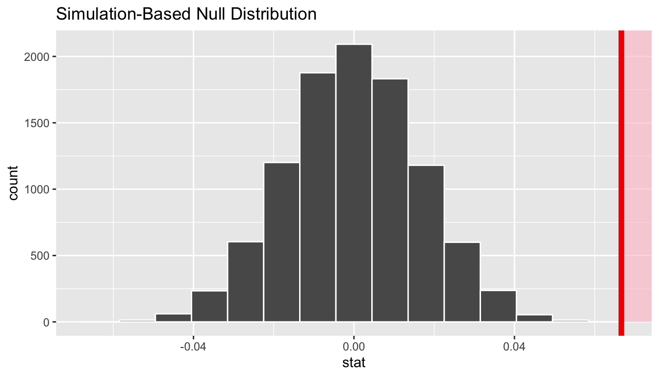

In viewing the distribution above with shading to the right of our observed slope value of 0.067, we can see that we expect the p-value to be quite small. Let’s calculate it next using a similar syntax to what was done with visualize().

11.1.7 The p-value

null_slope_distn %>% 
  get_pvalue(obs_stat = slope_obs, direction = "greater")

# A tibble: 1 x 1
  p_value
    <dbl>
1       0

Since 0.067 falls far to the right of this plot beyond where any of the histogram bins have data, we can say that we have a \(p\)-value of 0. We, thus, have evidence to reject the null hypothesis in support of there being a positive association between the beauty score and teaching score of University of Texas faculty members.

Learning check

(LC11.1) Repeat the inference above but this time for the correlation coefficient instead of the slope. Note the implementation of stat = "correlation" in the calculate() function of the infer package.

---

11.2 Bootstrapping for the regression slope

With the p-value calculated as 0 in the hypothesis test above, we can next determine just how strong of a positive slope value we might expect between the variables of teaching score and beauty score (bty_avg) for University of Texas faculty. Recall the infer pipeline above to compute the null distribution. Recall that this assumes the null hypothesis is true that there is no relationship between teaching score and beauty score using the hypothesize() function.

null_slope_distn <- evals %>% 
  specify(score ~ bty_avg) %>%
  hypothesize(null = "independence") %>% 
  generate(reps = 10000, type = "permute") %>% 
  calculate(stat = "slope")

To further reinforce the process being done in the pipeline, we’ve added the type argument to generate(). This is automatically added based on the entries for specify() and hypothesize() but it provides a useful way to check to make sure generate() is created the samples in the desired way. In this case, we permuted the values of one variable across the values of the other 10,000 times and calculated a "slope" coefficient for each of these 10,000 generated samples.

If instead we’d like to get a range of plausible values for the true slope value, we can use the process of bootstrapping:

bootstrap_slope_distn <- evals %>% 
  specify(score ~ bty_avg) %>%
  generate(reps = 10000, type = "bootstrap") %>% 
  calculate(stat = "slope")

bootstrap_slope_distn %>% visualize()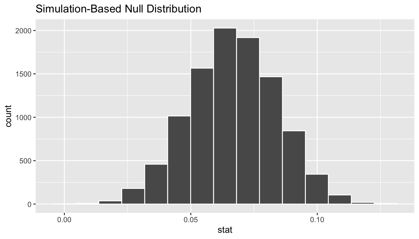

Next we can use the get_ci() function to determine the confidence interval. Let’s do this in two different ways obtaining 99% confidence intervals. Remember that these denote a range of plausible values for an unknown true population slope parameter regressing teaching score on beauty score.

percentile_slope_ci <- bootstrap_slope_distn %>% 
  get_ci(level = 0.99, type = "percentile")
percentile_slope_ci

# A tibble: 1 x 2
  `0.5%` `99.5%`
   <dbl>   <dbl>
1 0.0229   0.110

se_slope_ci <- bootstrap_slope_distn %>% 
  get_ci(level = 0.99, type = "se", point_estimate = slope_obs)
se_slope_ci

# A tibble: 1 x 2
   lower upper
   <dbl> <dbl>
1 0.0220 0.111

With the bootstrap distribution being close to symmetric, it makes sense that the two resulting confidence intervals are similar.

---

11.3 Inference for multiple regression

11.3.1 Refresher: Professor evaluations data

Let’s revisit the professor evaluations data that we analyzed using multiple regression with one numerical and one categorical predictor. In particular

• \(y\): outcome variable of instructor evaluation score
• predictor variables
  • \(x_1\): numerical explanatory/predictor variable of age
  • \(x_2\): categorical explanatory/predictor variable of gender

library(ggplot2)
library(dplyr)
library(moderndive)

evals_multiple <- evals %>%
  select(score, ethnicity, gender, language, age, bty_avg, rank)

First, recall that we had two competing potential models to explain professors’ teaching scores:

1. Model 1: No interaction term. i.e. both male and female profs have the same slope describing the associated effect of age on teaching score
2. Model 2: Includes an interaction term. i.e. we allow for male and female profs to have different slopes describing the associated effect of age on teaching score

11.3.2 Refresher: Visualizations

Recall the plots we made for both these models:

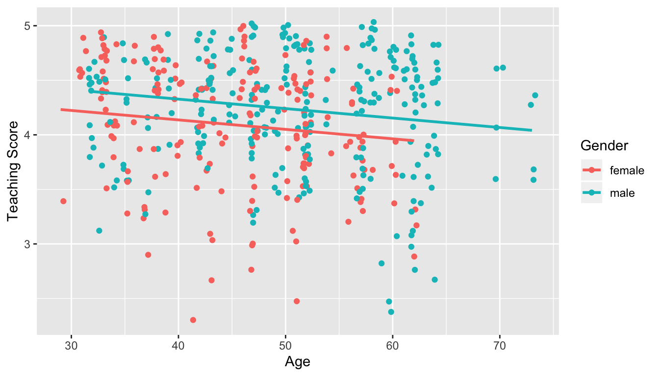
FIGURE 11.1: Model 1: no interaction effect included

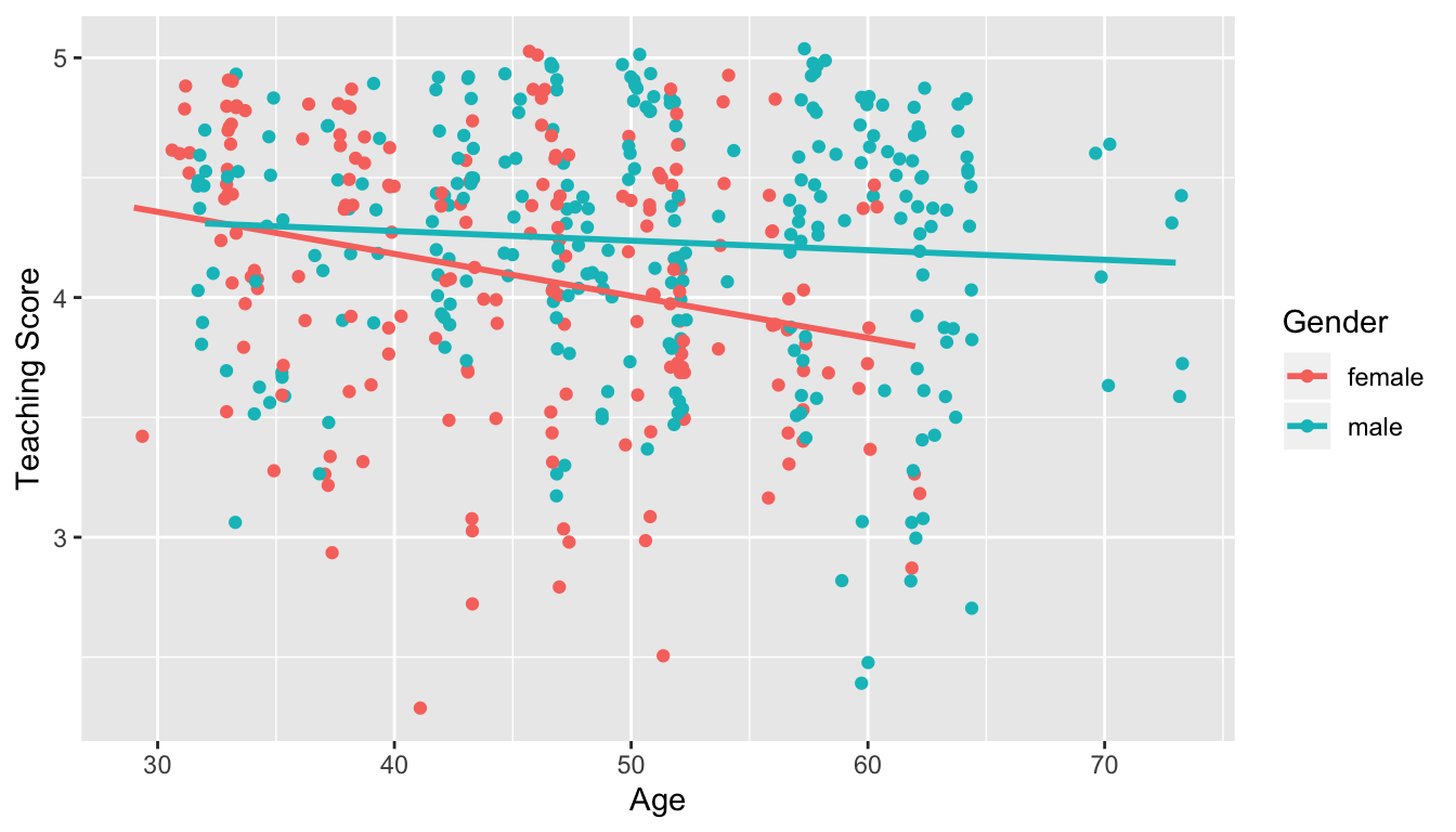
FIGURE 11.2: Model 2: interaction effect included

11.3.3 Refresher: Regression tables

Last, let’s recall the regressions we fit. First, the regression with no interaction effect: note the use of + in the formula in Table 11.1.

score_model_2 <- lm(score ~ age + gender, data = evals_multiple)
get_regression_table(score_model_2)

TABLE 11.1: Model 1: Regression table with no interaction effect included

term	estimate	std_error	statistic	p_value	lower_ci	upper_ci
intercept	4.484	0.125	35.79	0.000	4.238	4.730
age	-0.009	0.003	-3.28	0.001	-0.014	-0.003
gendermale	0.191	0.052	3.63	0.000	0.087	0.294

Second, the regression with an interaction effect: note the use of * in the formula.

score_model_3 <- lm(score ~ age * gender, data = evals_multiple)
get_regression_table(score_model_3)

TABLE 11.2: Model 2: Regression table with interaction effect included

term	estimate	std_error	statistic	p_value	lower_ci	upper_ci
intercept	4.883	0.205	23.80	0.000	4.480	5.286
age	-0.018	0.004	-3.92	0.000	-0.026	-0.009
gendermale	-0.446	0.265	-1.68	0.094	-0.968	0.076
age:gendermale	0.014	0.006	2.45	0.015	0.003	0.024

11.3.4 Script of R code

An R script file of all R code used in this chapter is available here.

---

11.4 Residual analysis

11.4.1 Residual analysis

Recall the residuals can be thought of as the error or the “lack-of-fit” between the observed value \(y\) and the fitted value \(\widehat{y}\) on the blue regression line in Figure 6.6. Ideally when we fit a regression model, we’d like there to be no systematic pattern to these residuals. We’ll be more specific as to what we mean by no systematic pattern when we see Figure 11.4 below, but let’s keep this notion imprecise for now. Investigating any such patterns is known as residual analysis and is the theme of this section.

We’ll perform our residual analysis in two ways:

1. Creating a scatterplot with the residuals on the \(y\)-axis and the original explanatory variable \(x\) on the \(x\)-axis.
2. Creating a histogram of the residuals, thereby showing the distribution of the residuals.

First, recall in Figure 6.8 above we created a scatterplot where

• on the vertical axis we had the teaching score \(y\),
• on the horizontal axis we had the beauty score \(x\), and
• the blue arrow represented the residual for one particular instructor.

Instead, in Figure 11.3 below, let’s create a scatterplot where

• On the vertical axis we have the residual \(y-\widehat{y}\) instead
• On the horizontal axis we have the beauty score \(x\) as before:

# Get data
evals_ch6 <- evals %>%
  select(score, bty_avg, age)
# Fit regression model:
score_model <- lm(score ~ bty_avg, data = evals_ch6)
# Get regression table:
get_regression_table(score_model)

# A tibble: 2 x 7
  term      estimate std_error statistic p_value lower_ci upper_ci
  <chr>        <dbl>     <dbl>     <dbl>   <dbl>    <dbl>    <dbl>
1 intercept    3.88      0.076     51.0        0    3.73     4.03 
2 bty_avg      0.067     0.016      4.09       0    0.035    0.099

# Get regression points
regression_points <- get_regression_points(score_model)

ggplot(regression_points, aes(x = bty_avg, y = residual)) +
  geom_point() +
  labs(x = "Beauty Score", y = "Residual") +
  geom_hline(yintercept = 0, col = "blue", size = 1)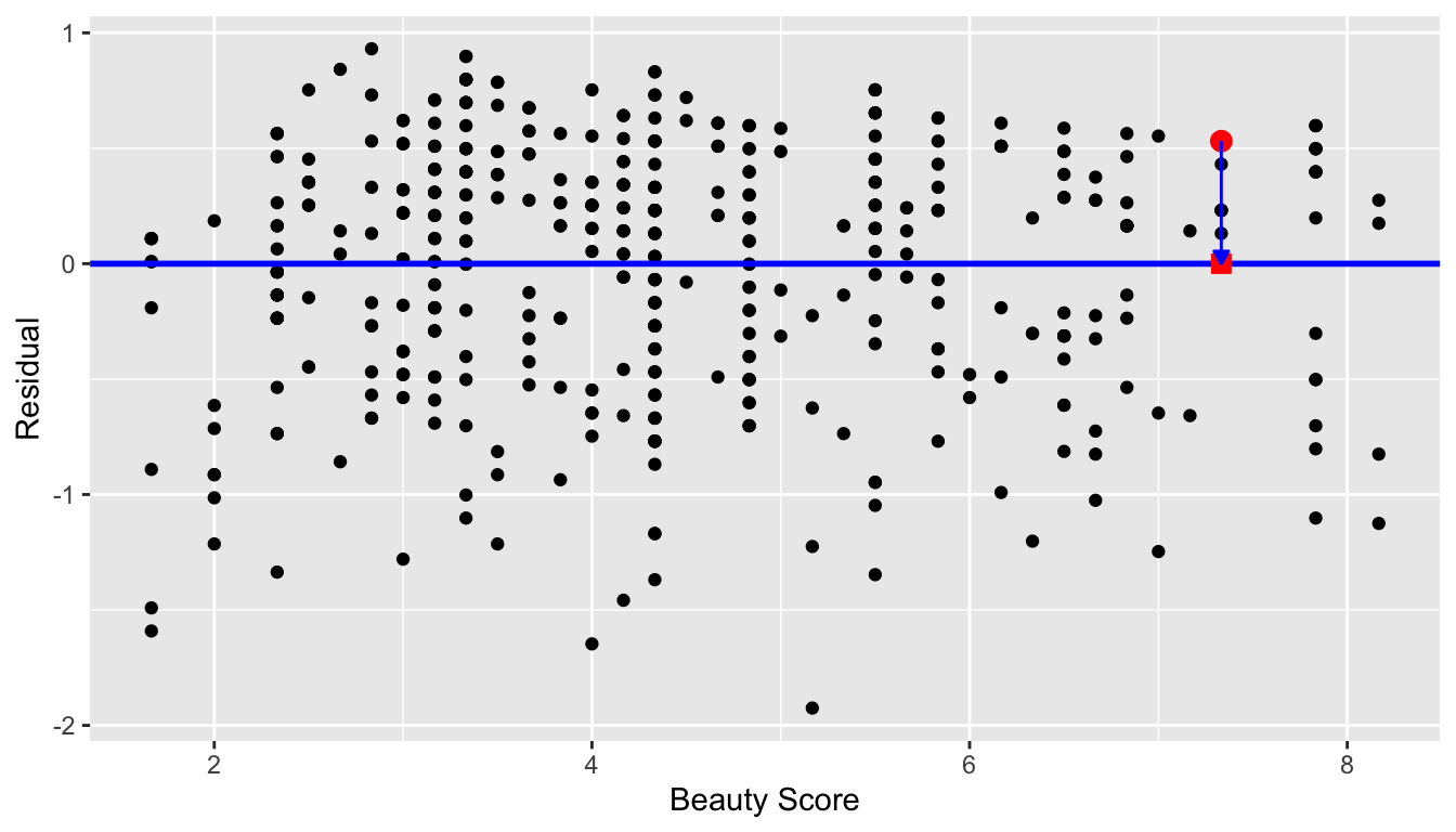

FIGURE 11.3: Plot of residuals over beauty score

You can think of Figure 11.3 as Figure 6.8 but with the blue line flattened out to \(y=0\). Does it seem like there is no systematic pattern to the residuals? This question is rather qualitative and subjective in nature, thus different people may respond with different answers to the above question. However, it can be argued that there isn’t a drastic pattern in the residuals.

Let’s now get a little more precise in our definition of no systematic pattern in the residuals. Ideally, the residuals should behave randomly. In addition,

1. the residuals should be on average 0. In other words, sometimes the regression model will make a positive error in that \(y - \widehat{y} > 0\), sometimes the regression model will make a negative error in that \(y - \widehat{y} < 0\), but on average the error is 0.
2. Further, the value and spread of the residuals should not depend on the value of \(x\).

In Figure 11.4 below, we display some hypothetical examples where there are drastic patterns to the residuals. In Example 1, the value of the residual seems to depend on \(x\): the residuals tend to be positive for small and large values of \(x\) in this range, whereas values of \(x\) more in the middle tend to have negative residuals. In Example 2, while the residuals seem to be on average 0 for each value of \(x\), the spread of the residuals varies for different values of \(x\); this situation is known as heteroskedasticity.

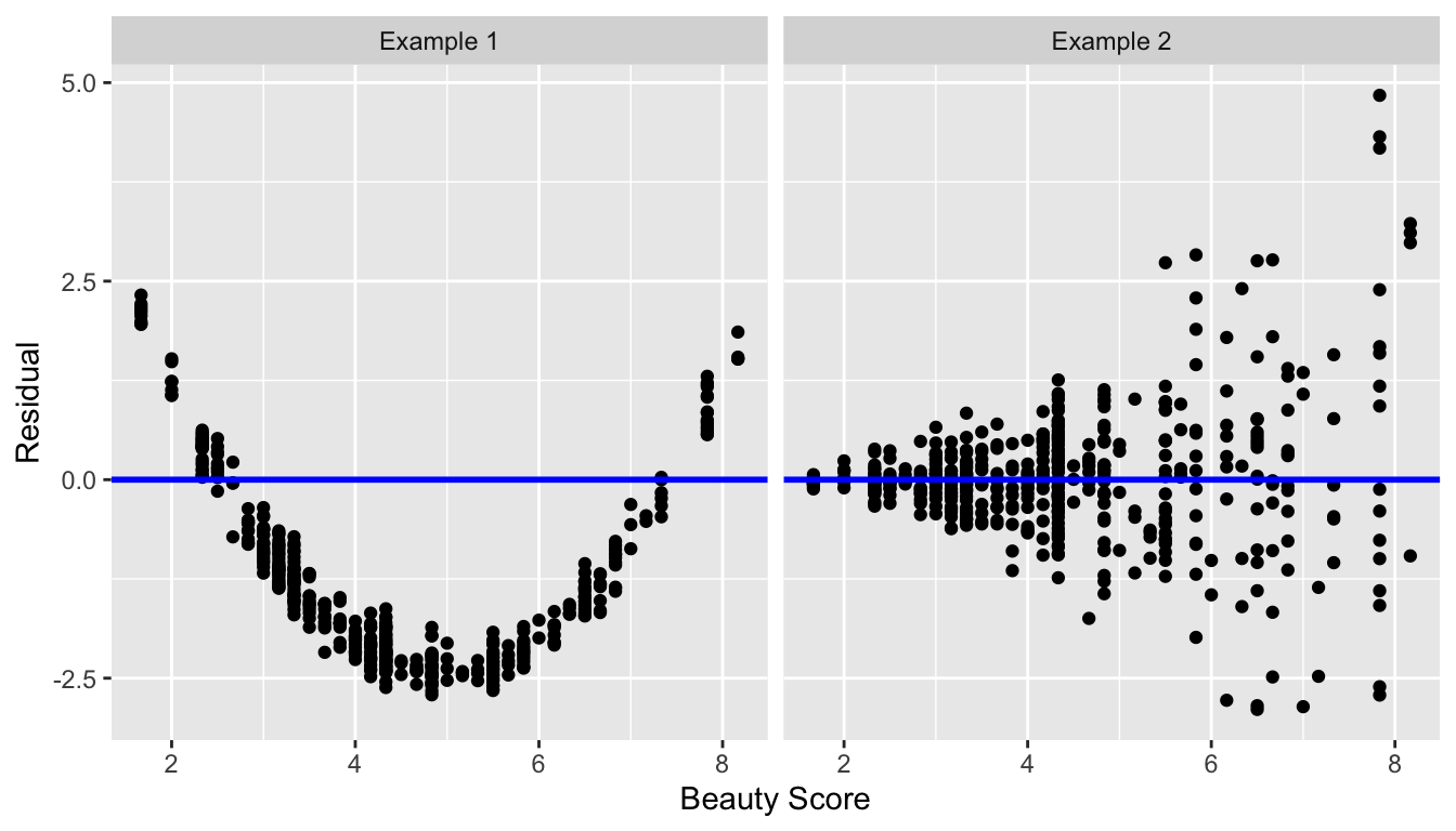
FIGURE 11.4: Examples of less than ideal residual patterns

The second way to perform a residual analysis is to look at the histogram of the residuals:

ggplot(regression_points, aes(x = residual)) +
  geom_histogram(binwidth = 0.25, color = "white") +
  labs(x = "Residual")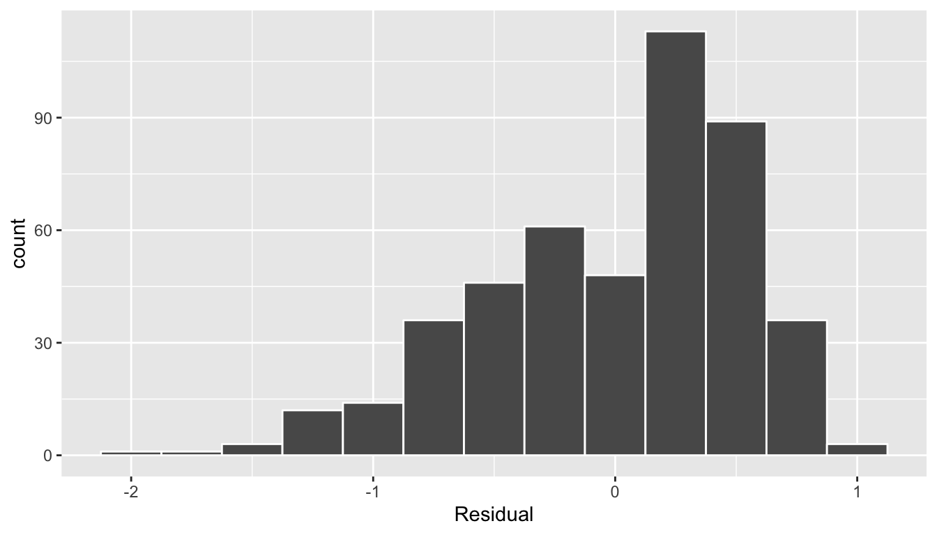

FIGURE 11.5: Histogram of residuals

This histogram seems to indicate that we have more positive residuals than negative. Since the residual \(y-\widehat{y}\) is positive when \(y > \widehat{y}\), it seems our fitted teaching score from the regression model tends to underestimate the true teaching score. This histogram has a slight left-skew in that there is a long tail on the left. Another way to say this is this data exhibits a negative skew. Is this a problem? Again, there is a certain amount of subjectivity in the response. In the authors’ opinion, while there is a slight skew/pattern to the residuals, it isn’t a large concern. On the other hand, others might disagree with our assessment. Here are examples of an ideal and less than ideal pattern to the residuals when viewed in a histogram:

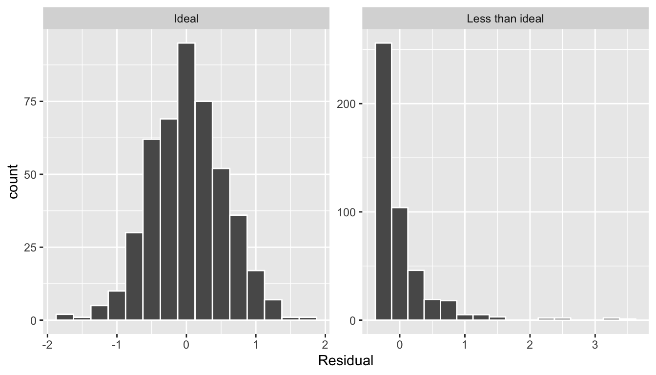
FIGURE 11.6: Examples of ideal and less than ideal residual patterns

In fact, we’ll see later on that we would like the residuals to be normally distributed with mean 0. In other words, be bell-shaped and centered at 0! While this requirement and residual analysis in general may seem to some of you as not being overly critical at this point, we’ll see later after when we cover inference for regression in Chapter 11 that for the last five columns of the regression table from earlier (std error, statistic, p_value,lower_ci, and upper_ci) to have valid interpretations, the above three conditions should roughly hold.

Learning check

(LC11.2) Continuing with our regression using age as the explanatory variable and teaching score as the outcome variable, use the get_regression_points() function to get the observed values, fitted values, and residuals for all 463 instructors. Perform a residual analysis and look for any systematic patterns in the residuals. Ideally, there should be little to no pattern.

11.4.2 Residual analysis

# Get data:
gapminder2007 <- gapminder %>%
  filter(year == 2007) %>% 
  select(country, continent, lifeExp, gdpPercap)
# Fit regression model:
lifeExp_model <- lm(lifeExp ~ continent, data = gapminder2007)
# Get regression table:
get_regression_table(lifeExp_model)

# A tibble: 5 x 7
  term              estimate std_error statistic p_value lower_ci upper_ci
  <chr>                <dbl>     <dbl>     <dbl>   <dbl>    <dbl>    <dbl>
1 intercept             54.8      1.02     53.4        0     52.8     56.8
2 continentAmericas     18.8      1.8      10.4        0     15.2     22.4
3 continentAsia         15.9      1.65      9.68       0     12.7     19.2
4 continentEurope       22.8      1.70     13.5        0     19.5     26.2
5 continentOceania      25.9      5.33      4.86       0     15.4     36.4

# Get regression points
regression_points <- get_regression_points(lifeExp_model)

Recall our discussion on residuals from Section 11.4.1 where our goal was to investigate whether or not there was a systematic pattern to the residuals. Ideally since residuals can be thought of as error, there should be no such pattern. While there are many ways to do such residual analysis, we focused on two approaches based on visualizations.

1. A plot with residuals on the vertical axis and the predictor (in this case continent) on the horizontal axis
2. A histogram of all residuals

First, let’s plot the residuals versus continent in Figure 11.7, but also let’s plot all 142 points with a little horizontal random jitter by setting the width = 0.1 parameter in geom_jitter():

ggplot(regression_points, aes(x = continent, y = residual)) +
  geom_jitter(width = 0.1) + 
  labs(x = "Continent", y = "Residual") +
  geom_hline(yintercept = 0, col = "blue")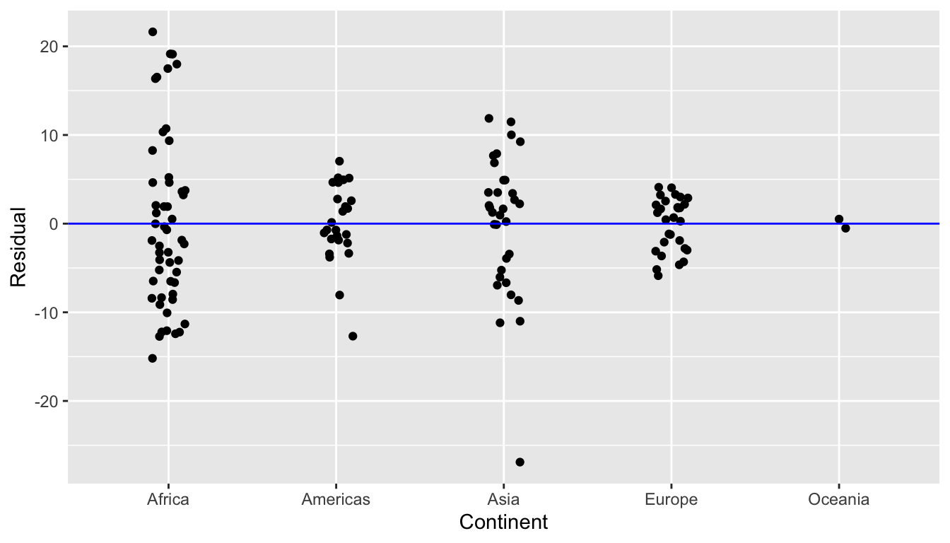

FIGURE 11.7: Plot of residuals over continent

We observe

1. There seems to be a rough balance of both positive and negative residuals for all 5 continents.
2. However, there is one clear outlier in Asia, which has a residual with the largest deviation away from 0.

Let’s investigate the 5 countries in Asia with the shortest life expectancy:

gapminder2007 %>%
  filter(continent == "Asia") %>%
  arrange(lifeExp)

TABLE 11.3: Countries in Asia with shortest life expectancy

country	continent	lifeExp	gdpPercap
Afghanistan	Asia	43.8	975
Iraq	Asia	59.5	4471
Cambodia	Asia	59.7	1714
Myanmar	Asia	62.1	944
Yemen, Rep.	Asia	62.7	2281

This was the earlier identified residual for Afghanistan of -26.9. Unfortunately given recent geopolitical turmoil, individuals who live in Afghanistan and, in particular in 2007, have a drastically lower life expectancy.

Second, let’s look at a histogram of all 142 values of residuals in Figure 11.8. In this case, the residuals form a rather nice bell-shape, although there are a couple of very low and very high values at the tails. As we said previously, searching for patterns in residuals can be somewhat subjective, but ideally we hope there are no “drastic” patterns.

ggplot(regression_points, aes(x = residual)) +
  geom_histogram(binwidth = 5, color = "white") +
  labs(x = "Residual")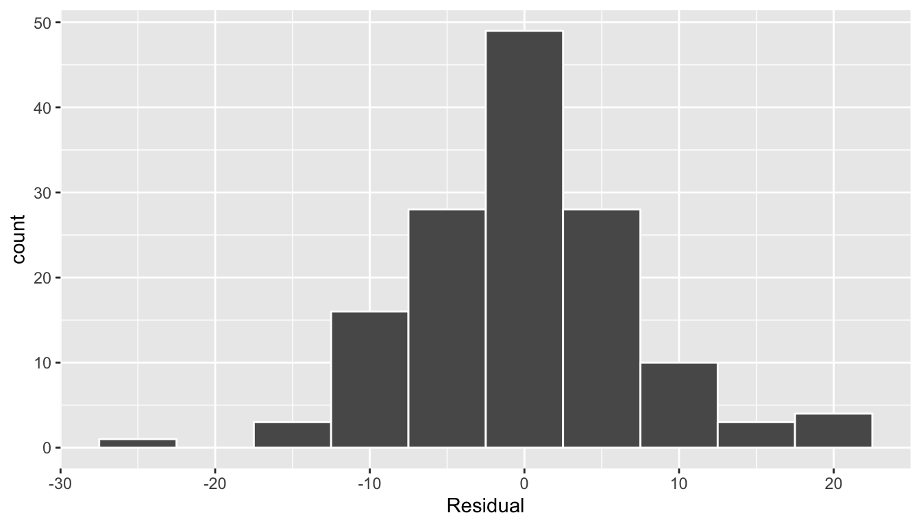

FIGURE 11.8: Histogram of residuals

Learning check

(LC11.3) Continuing with our regression using gdpPercap as the outcome variable and continent as the explanatory variable, use the get_regression_points() function to get the observed values, fitted values, and residuals for all 142 countries in 2007 and perform a residual analysis to look for any systematic patterns in the residuals. Is there a pattern? Please keep in mind that these types of questions are somewhat subjective and different people will most likely have different answers. The focus should be on being able to justify the conclusions made.

11.4.3 Residual analysis

Recall in Section 11.4.1, our first residual analysis plot investigated the presence of any systematic pattern in the residuals when we had a single numerical predictor: bty_age. For the Credit card dataset, since we have two numerical predictors, Limit and Income, we must perform this twice:

# Get data:
Credit <- Credit %>%
  select(Balance, Limit, Income, Rating, Age)
# Fit regression model:
Balance_model <- lm(Balance ~ Limit + Income, data = Credit)
# Get regression table:
get_regression_table(Balance_model)

# A tibble: 3 x 7
  term      estimate std_error statistic p_value lower_ci upper_ci
  <chr>        <dbl>     <dbl>     <dbl>   <dbl>    <dbl>    <dbl>
1 intercept -385.       19.5       -19.8       0 -423.    -347.   
2 Limit        0.264     0.006      45.0       0    0.253    0.276
3 Income      -7.66      0.385     -19.9       0   -8.42    -6.91 

# Get regression points
regression_points <- get_regression_points(Balance_model)

ggplot(regression_points, aes(x = Limit, y = residual)) +
  geom_point() +
  labs(x = "Credit limit (in $)", 
       y = "Residual", 
       title = "Residuals vs credit limit")
  
ggplot(regression_points, aes(x = Income, y = residual)) +
  geom_point() +
  labs(x = "Income (in $1000)", 
       y = "Residual", 
       title = "Residuals vs income")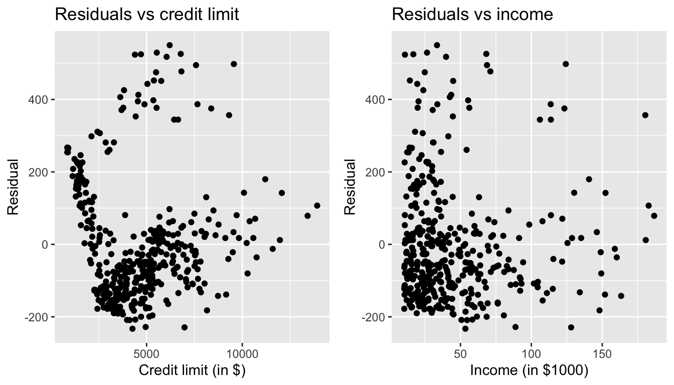

FIGURE 11.9: Residuals vs credit limit and income

In this case, there does appear to be a systematic pattern to the residuals. As the scatter of the residuals around the line \(y=0\) is definitely not consistent. This behavior of the residuals is further evidenced by the histogram of residuals in Figure 11.10. We observe that the residuals have a slight right-skew (recall we say that data is right-skewed, or positively-skewed, if there is a tail to the right). Ideally, these residuals should be bell-shaped around a residual value of 0.

ggplot(regression_points, aes(x = residual)) +
  geom_histogram(color = "white") +
  labs(x = "Residual")

`stat_bin()` using `bins = 30`. Pick better value with `binwidth`.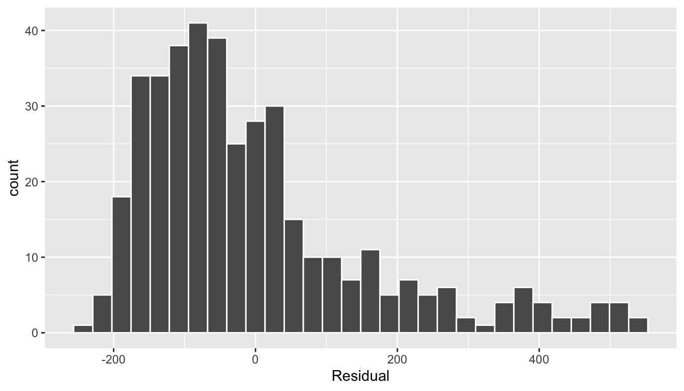

FIGURE 11.10: Relationship between credit card balance and credit limit/income

Another way to interpret this histogram is that since the residual is computed as \(y - \widehat{y}\) = balance - balance_hat, we have some values where the fitted value \(\widehat{y}\) is very much lower than the observed value \(y\). In other words, we are underestimating certain credit card holders’ balances by a very large amount.

Learning check

(LC11.4) Continuing with our regression using Rating and Age as the explanatory variables and credit card Balance as the outcome variable, use the get_regression_points() function to get the observed values, fitted values, and residuals for all 400 credit card holders. Perform a residual analysis and look for any systematic patterns in the residuals.

11.4.4 Residual analysis

# Get data:
evals_ch7 <- evals %>%
  select(score, age, gender)
# Fit regression model:
score_model_2 <- lm(score ~ age + gender, data = evals_ch7)
# Get regression table:
get_regression_table(score_model_2)

# A tibble: 3 x 7
  term       estimate std_error statistic p_value lower_ci upper_ci
  <chr>         <dbl>     <dbl>     <dbl>   <dbl>    <dbl>    <dbl>
1 intercept     4.48      0.125     35.8    0        4.24     4.73 
2 age          -0.009     0.003     -3.28   0.001   -0.014   -0.003
3 gendermale    0.191     0.052      3.63   0        0.087    0.294

# Get regression points
regression_points <- get_regression_points(score_model_2)

As always, let’s perform a residual analysis first with a histogram, which we can facet by gender:

ggplot(regression_points, aes(x = residual)) +
  geom_histogram(binwidth = 0.25, color = "white") +
  labs(x = "Residual") +
  facet_wrap(~gender)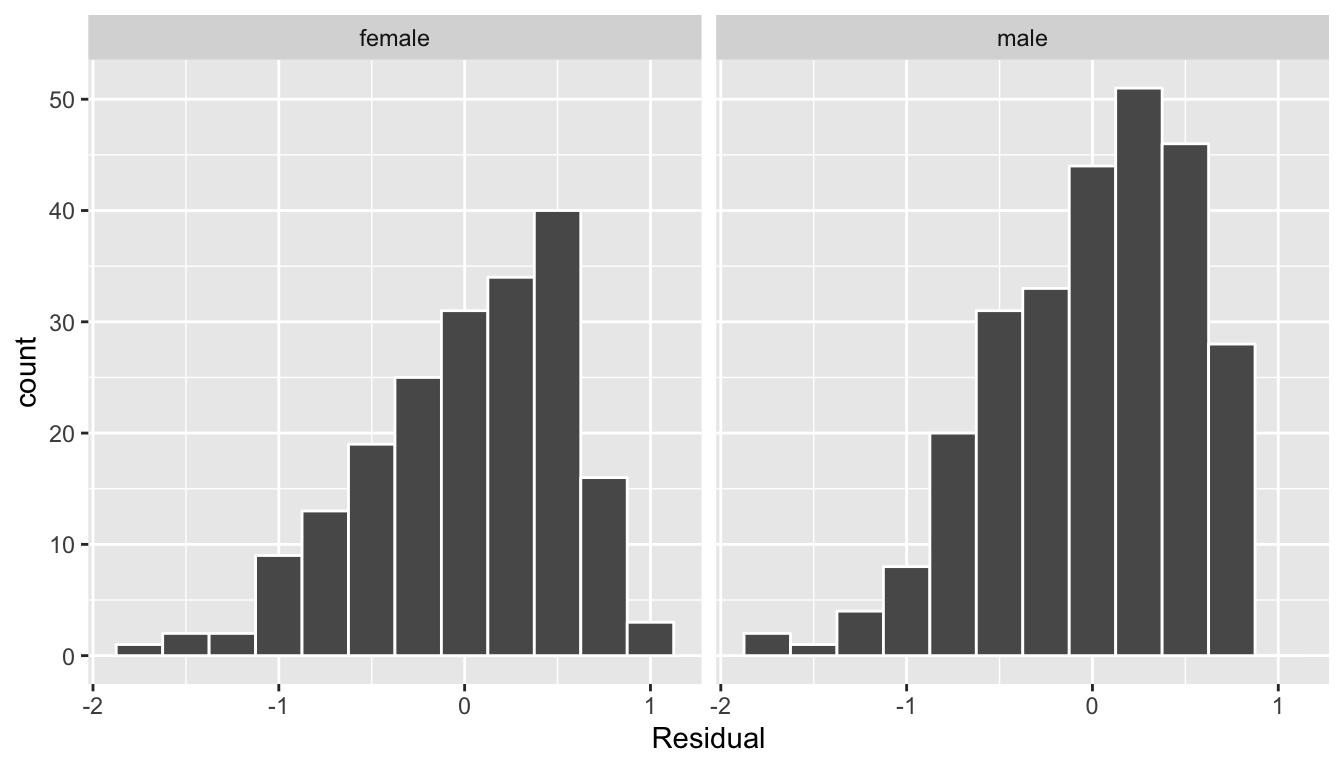

FIGURE 11.11: Interaction model histogram of residuals

Second, the residuals as compared to the predictor variables:

• \(x_1\): numerical explanatory/predictor variable of age
• \(x_2\): categorical explanatory/predictor variable of gender

ggplot(regression_points, aes(x = age, y = residual)) +
  geom_point() +
  labs(x = "age", y = "Residual") +
  geom_hline(yintercept = 0, col = "blue", size = 1) +
  facet_wrap(~ gender)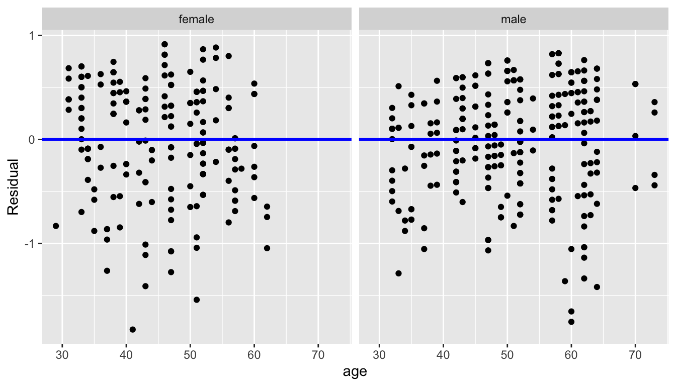

FIGURE 11.12: Interaction model residuals vs predictor