5 Data Manipulation via dplyr
Let’s briefly recap where we have been so far and where we are headed. In Chapter 3, we discussed what it means for data to be tidy. We saw that this refers to observational units corresponding to rows and variables being stored in columns (one variable for every column). The entries in the data frame correspond to different combinations of observational units and variables. In the flights data frame, we saw that each row corresponds to a different flight leaving New York City. In other words, the observational unit of that tidy data frame is a flight. The variables are listed as columns and for flights they include both quantitative variables like dep_delay and distance but also categorical variables like carrier and origin. An entry in the table corresponds to a particular flight on a given day and a particular value of a given variable representing that flight.
We saw in Chapter 4 that organizing data in this tidy way makes it easy for us to produce graphics. We can simply specify what variable/column we would like on one axis, what variable we’d like on the other axis, and what type of plot we’d like to make. We can also do things such as changing the color by another variable or change the size of our points by a fourth variable given this tidy data set.
Furthermore, in Chapter 4, we hinted at some ways to summarize and manipulate data to suit your needs. This chapter expands on this by giving a variety of examples using what we call the Five Main Verbs in the dplyr package (Wickham et al. 2017). There are more advanced operations than just these and you’ll see some examples of this near the end of the chapter.
While at various points we specifically make mention to use the View() command to inspect a particular data frame, feel free to do so whenever. In fact, you should get into the habit of doing this for any data frame you work with.
Needed packages
Before we proceed with this chapter, let’s load all the necessary packages.
library(dplyr)
library(ggplot2)
library(nycflights13)
library(knitr)
5.1 The pipe %>%
Before we introduce the five main verbs, we first introduce the the pipe operator (%>%). Just as the + sign was used to add layers to a plot created using ggplot(), the pipe operator allows us to chain together dplyr data manipulation functions. The pipe operator can be read as “then”. The %>% operator allows us to go from one step in dplyr to the next easily so we can, for example:
filterour data frame to only focus on a few rows thengroup_byanother variable to create groups thensummarizethis grouped data to calculate the mean for each level of the group.
The piping syntax will be our major focus throughout the rest of this book and you’ll find that you’ll quickly be addicted to the chaining with some practice. If you’d like to see more examples on using dplyr, the 5MV (in addition to some other dplyr verbs), and %>% with the nycflights13 data set, you can check out Chapter 5 of Hadley and Garrett’s book (Grolemund and Wickham 2016).
5.2 Five Main Verbs - The 5MV
The d in dplyr stands for data frames, so the functions here work when you are working with objects of the data frame type. It’s most important for you to focus on the 5MV: the five most commonly used functions that help us manipulate and summarize data. A description of these verbs follows with each subsection devoted to seeing an example of that verb in play (or a combination of a few verbs):
filter: Pick rows based on conditions about their valuessummarize: Create summary measures of variables either- over the entire data frame
- or over groups of observations on variables using
group_by
mutate: Create a new variable in the data frame by mutating existing onesarrange: Arrange/sort the rows based on one or more variables
Just as we had the 5NG (The Five Named Graphs in Chapter 4 using ggplot2) for data visualization, we also have the 5MV here (The Five Main Verbs in dplyr) for data manipulation. All of the 5MVs follow the same syntax with the argument before the pipe %>% being the name of the data frame and then the name of the verb with other arguments specifying which criteria you’d like the verb to work with in parentheses.
5.2.1 5MV#1: Filter observations using filter

Figure 5.1: Filter diagram from Data Wrangling with dplyr and tidyr cheatsheet
The filter function here works much like the “Filter” option in Microsoft Excel; it allows you to specify criteria about values of a variable in your data set and then chooses only those rows that match that criteria. We begin by focusing only on flights from New York City to Portland, Oregon. The dest code (or airport code) for Portland, Oregon is "PDX". Run the following and look at the resulting spreadsheet to ensure that only flights heading to Portland are chosen here:
portland_flights <- flights %>%
  filter(dest == "PDX")
View(pdx_flights)
Note the following:
- The ordering of the commands:
- Take the data frame
flightsthen filterthe data frame so that only those where thedestequals"PDX"are included.
- Take the data frame
- The double equal sign
==You are almost guaranteed to make the mistake at least once of only including one equals sign. Let’s see what happens when we make this error:
portland_flights <- flights %>%
  filter(dest = "PDX")
Error: filter() takes unnamed arguments. Do you need `==`?You can combine multiple criteria together using operators that make comparisons:
|corresponds to “or”&corresponds to “and”
We can often skip the use of & and just separate our conditions with a comma. You’ll see this in the example below.
In addition, you can use other mathematical checks (similar to ==):
>corresponds to “greater than”<corresponds to “less than”>=corresponds to “greater than or equal to”<=corresponds to “less than or equal to”!=corresponds to “not equal to”
To see many of these in action, let’s select all flights that left JFK airport heading to Burlington, Vermont ("BTV") or Seattle, Washington ("SEA") in the months of October, November, or December. Run the following
btv_sea_flights_fall <- flights %>%
  filter(origin == "JFK", (dest == "BTV" | dest == "SEA"), month >= 10)
View(btv_sea_flights_fall)
Note how even though colloquially speaking one might say “all flights leaving Burlington, Vermont and Seattle, Washington”, in terms of computer operations, we really mean “all flights leaving Burlington, Vermont or Seattle, Washington”, because for a given row in the data, dest can either be: “BTV”, “SEA”, or something else, but not “BTV” and “SEA” at the same time.
Another example uses the ! to pick rows that DON’T match a condition. Here we are selecting rows corresponding to flights that didn’t go to Burlington, VT or Seattle, WA.
not_BTV_SEA <- flights %>%
  filter(!(dest == "BTV" | dest == "SEA"))
View(not_BTV_SEA)
As a final note we point out that filter() should often be the first verb you’ll apply to your data. This cleans your data set to only those rows you care about, or put differently, it narrows down the scope to just the observational units your care about.
Learning check
(LC5.1) What’s another way using ! we could filter only the rows that are not going to Burlington, VT nor Seattle, WA in the flights data frame? Test this out using the code above.
5.2.2 5MV#2: Summarize variables using summarize

Figure 5.2: Summarize diagram from Data Wrangling with dplyr and tidyr cheatsheet

Figure 5.3: Another summarize diagram from Data Wrangling with dplyr and tidyr cheatsheet
We saw in Subsection ?? a way to calculate the standard deviation and mean of the temperature variable temp in the weather data frame of nycflights. We can do so in one step using the summarize function in dplyr:
summary_temp <- weather %>%
  summarize(mean = mean(temp), std_dev = sd(temp))
summary_temp
## # A tibble: 1 x 2
## mean std_dev
## <dbl> <dbl>
## 1 NA NAWe’ve created a small data frame here called summary_temp that includes both the mean and the std_dev of the temp variable in weather. Notice as shown in Figures 5.2 and 5.3, the data frame weather went from many rows to a single row of just the summary values in the data frame summary_temp. But why are the mean and standard deviation missing, i.e. NA? Remember that by default the mean and sd functions do not ignore missing values. We need to specify the argument na.rm=TRUE (rm is short for “remove”):
summary_temp <- weather %>%
  summarize(mean = mean(temp, na.rm = TRUE), std_dev = sd(temp, na.rm = TRUE))
summary_temp
## # A tibble: 1 x 2
## mean std_dev
## <dbl> <dbl>
## 1 55.20351 17.78212If we’d like to access either of these values directly we can use the $ to specify a column in a data frame. For example:
summary_temp$mean## [1] 55.20351You’ll often encounter issues with missing values NA. In fact, an entire branch of the field of statistics deals with missing data. However, it is not good practice to include a na.rm = TRUE in your summary commands by default; you should attempt to run them without this argument. The idea being you should at the very least be alerted to the presence of missing values and consider what the impact on the analysis might be if you ignore these values. In other words, na.rm = TRUE should only be used when necessary.
What other summary functions can we use inside the summarize() verb? Any function in R that takes a vector of values and returns just one. Here are just a few:
min()andmax(): the minimum and maximum values respectivelyIQR(): Interquartile rangesum(): the sumn(): a count of the number of rows/observations in each group. This particular summary function will make more sense in thegroup_bychapter.
Learning check
(LC5.2) Say a doctor is studying the effect of smoking on lung cancer of a large number of patients who have records measured at five year intervals. He notices that a large number of patients have missing data points because the patient has died, so he chooses to ignore these patients in his analysis. What is wrong with this doctor’s approach?
(LC5.3) Modify the above summarize function to be use the n() summary function: summarize(count=n()). What does the returned value correspond to?
(LC5.4) Why doesn’t the following code work? You may want to run the code line by line:
summary_temp <- weather %>%
  summarize(mean = mean(temp, na.rm = TRUE)) %>%
  summarize(std_dev = sd(temp, na.rm = TRUE))
5.2.3 5MV#3: Group rows using group_by
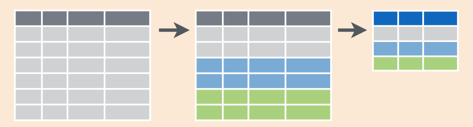
Figure 5.4: Group by and summarize diagram from Data Wrangling with dplyr and tidyr cheatsheet
However, it’s often more useful to summarize a variable based on the groupings of another variable. Let’s say similarly to the previous section, we are interested in the mean and standard deviation of temperatures but grouped by month. This concept can equivalently be articulated as: we want the mean and standard deviation of temperatures
- split by month.
- sliced by month.
- aggregated by month.
- collapsed over month.
We believe that you will be amazed at just how simple this is. Run the following code:
summary_monthly_temp <- weather %>%
  group_by(month) %>%
  summarize(mean = mean(temp, na.rm = TRUE),
            std_dev = sd(temp, na.rm = TRUE))
summary_monthly_temp
## # A tibble: 12 x 3
## month mean std_dev
## <dbl> <dbl> <dbl>
## 1 1 35.64127 10.185459
## 2 2 34.15454 6.940228
## 3 3 39.81404 6.224948
## 4 4 51.67094 8.785250
## 5 5 61.59185 9.608687
## 6 6 72.14500 7.603356
## 7 7 80.00967 7.147631
## 8 8 74.40495 5.171365
## 9 9 67.42582 8.475824
## 10 10 60.03305 8.829652
## 11 11 45.10893 10.502249
## 12 12 38.36811 9.940822This code is identical to the previous code that created summary_temp, but there is an extra group_by(month) spliced in between. By simply grouping the weather data set by month first and then passing this new data frame into summarize we get a resulting data frame that shows the mean and standard deviation temperature for each month in New York City. Since each row in summary_monthly_temp represents a summary of different rows in weather, the observational units have changed.
It is important to note that group_by doesn’t actually change the data frame. It simply sets meta-data (data about the data), specifically the group structure of the data. It is only after we apply the summarize function that the data frame actually changes. If we would like to remove this group structure meta-data, we can pipe a resulting data frame into the ungroup() function.
We now revisit the n() counting summary function we introduced in the previous section. For example, suppose we’d like to get a sense for how many flights departed each of the three airports in New York City:
by_origin <- flights %>%
  group_by(origin) %>%
  summarize(count = n())
by_origin
## # A tibble: 3 x 2
## origin count
## <chr> <int>
## 1 EWR 120835
## 2 JFK 111279
## 3 LGA 104662We see that Newark ("EWR") had the most flights departing in 2013 followed by "JFK" and lastly by LaGuardia ("LGA"). Note there is a subtle but important difference between sum() and n(). While sum() simply adds up a large set of numbers, the latter counts the number of times each of many different values occur.
You are not limited to grouping by one variable! Say you wanted to know the number of flights leaving each of the three New York City airports for each month, we can also group by a second variable month: group_by(origin, month). Run the following:
by_monthly_origin <- flights %>%
  group_by(origin, month) %>%
  summarize(count = n())
View(by_monthly_origin)
Learning check
(LC5.5) Recall from Chapter 4 when we looked at plots of temperatures by months in NYC. What does the standard deviation column in the summary_monthly_temp data frame tell us about temperatures in New York City throughout the year?
(LC5.6) What code would be required to get the mean and standard deviation temperature for each day in 2013 for NYC?
(LC5.7) Recreate by_monthly_origin, but instead of grouping via group_by(origin, month), group variables in a different order group_by(month, origin). What differs in the resulting data set?
(LC5.8) How could we identify how many flights left each of the three airports for each carrier?
(LC5.9) How does the filter operation differ from a group_by followed by a summarize?
5.2.4 5MV#4: Create new variables/change old variables using mutate
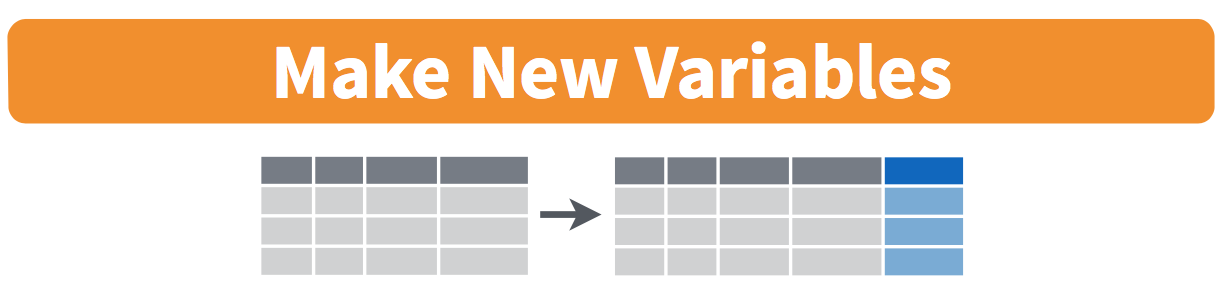
Figure 5.5: Mutate diagram from Data Wrangling with dplyr and tidyr cheatsheet
When looking at the flights data set, there are some clear additional variables that could be calculated based on the values of variables already in the data set. Passengers are often frustrated when their flights departs late, but change their mood a bit if pilots can make up some time during the flight to get them to their destination close to when they expected to land. This is commonly referred to as “gain” and we will create this variable using the mutate function. Note that we have also overwritten the flights data frame with what it was before as well as an additional variable gain here.
flights <- flights %>%
  mutate(gain = arr_delay - dep_delay)
Why did we overwrite flights instead of assigning the resulting data frame to a new object, like flights_with_gain? As a rough rule of thumb, as long as you are not losing information that you might need later, its acceptable practice to overwrite data frames. However, if you overwrite existing variables and/or change the observational units, recovering the original information might prove difficult. It this case, it might make sense to create a new data object.
Let’s look at summary measures of this gain variable and even plot it in the form of a histogram:
gain_summary <- flights %>%
  summarize(
    min = min(gain, na.rm = TRUE),
    q1 = quantile(gain, 0.25, na.rm = TRUE),
    median = quantile(gain, 0.5, na.rm = TRUE),
    q3 = quantile(gain, 0.75, na.rm = TRUE),
    max = max(gain, na.rm = TRUE),
    mean = mean(gain, na.rm = TRUE),
    sd = sd(gain, na.rm = TRUE),
    missing = sum(is.na(gain))
  )
gain_summary
## # A tibble: 1 x 8
## min q1 median q3 max mean sd missing
## <dbl> <dbl> <dbl> <dbl> <dbl> <dbl> <dbl> <int>
## 1 -109 -17 -7 3 196 -5.659779 18.04365 9430We’ve recreated the summary function we saw in Chapter 4 here using the summarize function in dplyr.
ggplot(data = flights, mapping = aes(x = gain)) +
  geom_histogram(color = "white", bins = 20)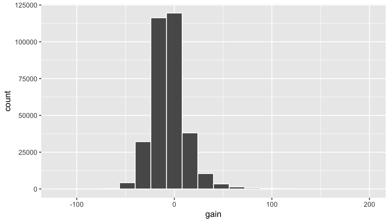
Figure 5.6: Histogram of gain variable
We can also create multiple columns at once and even refer to columns that were just created in a new column. Hadley produces one such example in Chapter 5 of “R for Data Science” (Grolemund and Wickham 2016):
flights <- flights %>%
  mutate(
    gain = arr_delay - dep_delay,
    hours = air_time / 60,
    gain_per_hour = gain / hours
  )
Learning check
(LC5.10) What do positive values of the gain variable in flights correspond to? What about negative values? And what about a zero value?
(LC5.11) Could we create the dep_delay and arr_delay columns by simply subtracting dep_time from sched_dep_time and similarly for arrivals? Try the code out and explain any differences between the result and what actually appears in flights.
(LC5.12) What can we say about the distribution of gain? Describe it in a few sentences using the plot and the gain_summary data frame values.
5.2.5 5MV#5: Reorder the data frame using arrange
As you may have thought about with the data frames we’ve worked with so far in the book, one of the most common things you’d like to do is sort the data frames by a specific variable in a column. Have you ever been asked to calculate a median by hand? This requires you to put the data in order from smallest to highest in value. The dplyr package has a function called arrange that we will use to sort/reorder our data according to the values of the specified variable. This is often used after we have used the group_by and summarize functions as we will see.
Let’s suppose we were interested in determining the most frequent destination airports from New York City in 2013:
freq_dest <- flights %>%
  group_by(dest) %>%
  summarize(num_flights = n())
freq_dest
## # A tibble: 105 x 2
## dest num_flights
## <chr> <int>
## 1 ABQ 254
## 2 ACK 265
## 3 ALB 439
## 4 ANC 8
## 5 ATL 17215
## 6 AUS 2439
## 7 AVL 275
## 8 BDL 443
## 9 BGR 375
## 10 BHM 297
## # ... with 95 more rowsYou’ll see that by default the values of dest are displayed in alphabetical order here. We are interested in finding those airports that appear most:
freq_dest %>% arrange(num_flights)## # A tibble: 105 x 2
## dest num_flights
## <chr> <int>
## 1 LEX 1
## 2 LGA 1
## 3 ANC 8
## 4 SBN 10
## 5 HDN 15
## 6 MTJ 15
## 7 EYW 17
## 8 PSP 19
## 9 JAC 25
## 10 BZN 36
## # ... with 95 more rowsThis is actually giving us the opposite of what we are looking for. It tells us the least frequent destination airports first. To switch the ordering to be descending instead of ascending we use the desc function:
freq_dest %>% arrange(desc(num_flights))## # A tibble: 105 x 2
## dest num_flights
## <chr> <int>
## 1 ORD 17283
## 2 ATL 17215
## 3 LAX 16174
## 4 BOS 15508
## 5 MCO 14082
## 6 CLT 14064
## 7 SFO 13331
## 8 FLL 12055
## 9 MIA 11728
## 10 DCA 9705
## # ... with 95 more rows5.3 Joining data frames
Another common task is joining/merging two different data sets. For example, in the flights data, the variable carrier lists the carrier code for the different flights. While "UA" and "AA" might be somewhat easy to guess for some (United and American Airlines), what are “VX”, “HA”, and “B6”? This information is provided in a separate data frame airlines.
View(airlines)We see that in airports, carrier is the carrier code while name is the full name of the airline. Using this table, we can see that “VX”, “HA”, and “B6” correspond to Virgin America, Hawaiian Airlines, and JetBlue respectively. However, will we have to continually look up the carrier’s name for each flight in the airlines data set? No! Instead of having to manually do this, we can have R automatically do this “looking up” for us.
Note that the values in the variable carrier in flights match the values in the variable carrier in airlines. In this case, we can use the variable carrier as a key variable to join/merge/match the two data frames by. Hadley and Garrett (Grolemund and Wickham 2016) created the following diagram to help us understand how the different data sets are linked:
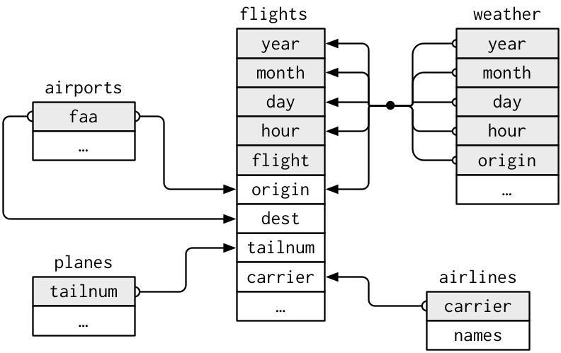
Figure 5.7: Data relationships in nycflights13 from R for Data Science
5.3.1 Joining by Key Variables
In both flights and airlines, the key variable we want to join/merge/match the two data frames with has the same name in both data sets: carriers. We make use of the inner_join() function to join by the variable carrier.
flights_joined <- flights %>%
  inner_join(airlines, by="carrier")
View(flights)
View(flights_joined)
We observed that the flights and flights_joined are identical except that flights_joined has an additional variable name whose values were drawn from airlines.
A visual representation of the inner_join is given below (Grolemund and Wickham 2016):
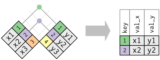
Figure 5.8: Diagram of inner join from R for Data Science
There are more complex joins available, but the inner_join will solve nearly all of the problems you’ll face in our experience.
5.3.2 Joining by Key Variables with Different Names
Say instead, you are interested in all the destinations of flights from NYC in 2013 and ask yourself:
- “What cities are these airports in?”
- “Is
"ORD"Orlando?” - “Where is
"FLL"?
The airports data frame contains airport codes:
View(airports)However, looking at both the airports and flights and the visual representation of the relations between the data frames in Figure 5.8, we see that in:
airportsthe airport code is in the variablefaaflightsthe airport code is in the variableorigin
So to join these two data sets, our inner_join operation involves a by argument that accounts for the different names:
flights %>%
  inner_join(airports, by = c("dest" = "faa"))
Let’s construct the sequence of commands that computes the number of flights from NYC to each destination but also includes information about each destination airport:
named_dests <- flights %>%
  group_by(dest) %>%
  summarize(num_flights = n()) %>%
  arrange(desc(num_flights)) %>%
  inner_join(airports, by = c("dest" = "faa")) %>%
  rename(airport_name = name)
View(named_dests)
In case you didn’t know, "ORD" is the airport code of Chicago O’Hare airport and "FLL" is the main airport in Fort Lauderdale, Florida, which we can now see in our named_freq_dests data frame.
Learning check
(LC5.13) Looking at Figure 5.7, when joining flights and weather, or in order words match the hourly weather values with each flight, why do we need to join by all of year, month, day, hour, and origin, and not just hour?
(LC5.14) What surprises you about the top 10 destinations from NYC in 2013?
5.4 Optional: Other verbs
5.4.1 Select variables using select

Figure 5.9: Select diagram from Data Wrangling with dplyr and tidyr cheatsheet
We’ve seen that the flights data frame in the nycflights13 package contains many different variables. The names function gives a listing of all the columns in a data frame; in our case you would run names(flights). You can also identify these variables by running the glimpse function in the dplyr package:
glimpse(flights)However, say you only want to consider two of these variables, say carrier and flight. You can select these:
flights %>%
  select(carrier, flight)
Another one of these variables is year. If you remember the original description of the flights data frame (or by running ?flights), you’ll remember that this data correspond to flights in 2013 departing New York City. The year variable isn’t really a variable here in that it doesn’t vary… flights actually comes from a larger data set that covers many years. We may want to remove the year variable from our data set since it won’t be helpful for analysis in this case. We can deselect year by using the - sign:
flights_no_year <- flights %>%
  select(-year)
names(flights_no_year)
Or we could specify a ranges of columns:
flight_arr_times <- flights %>%
  select(month:day, arr_time:sched_arr_time)
flight_arr_times
The select function can also be used to reorder columns in combination with the everything helper function. Let’s suppose we’d like the hour, minute, and time_hour variables, which appear at the end of the flights data set, to actually appear immediately after the day variable:
flights_reorder <- flights %>%
  select(month:day, hour:time_hour, everything())
names(flights_reorder)
in this case everything() picks up all remaining variables. Lastly, the helper functions starts_with, ends_with, and contains can be used to choose column names that match those conditions:
flights_begin_a <- flights %>%
  select(starts_with("a"))
flights_begin_a
flights_delays <- flights %>%
select(ends_with("delay"))
flights_delaysflights_time <- flights %>%
select(contains("time"))
flights_time5.4.2 Rename variables using rename
Another useful function is rename, which as you may suspect renames one column to another name. Suppose we wanted dep_time and arr_time to be departure_time and arrival_time instead in the flights_time data frame:
flights_time_new <- flights %>%
  select(contains("time")) %>%
  rename(departure_time = dep_time,
         arrival_time = arr_time)
names(flights_time)
It’s easy to forget if the new name comes before or after the equals sign. I usually remember this as “New Before, Old After” or NBOA. You’ll receive an error if you try to do it the other way:
Error: Unknown variables: departure_time, arrival_time.5.4.3 Find the top number of values using top_n
We can also use the top_n function which automatically tells us the most frequent num_flights. We specify the top 10 airports here:
named_dests %>%
  top_n(n = 10, wt = num_flights)
We’ll still need to arrange this by num_flights though:
named_dests  %>%
  top_n(n = 10, wt = num_flights) %>%
  arrange(desc(num_flights))
Note: Remember that I didn’t pull the n and wt arguments out of thin air. They can be found by using the ? function on top_n.
We can go one stop further and tie together the group_by and summarize functions we used to find the most frequent flights:
ten_freq_dests <- flights %>%
  group_by(dest) %>%
  summarize(num_flights = n()) %>%
  top_n(n = 10) %>%
  arrange(desc(num_flights))
View(ten_freq_dests)
Learning check
(LC5.15) What are some ways to select all three of the dest, air_time, and distance variables from flights? Give the code showing how to do this in at least three different ways.
(LC5.16) How could one use starts_with, ends_with, and contains to select columns from the flights data frame? Provide three different examples in total: one for starts_with, one for ends_with, and one for contains.
(LC5.17) Why might we want to use the select function on a data frame?
paste0("(LC", chap, ".", (lc <- lc + 1), ")") Create a new data frame that shows the top 5 airports with the largest arrival delays from NYC in 2013.
5.5 Conclusion
5.5.1 Resources
As we saw with the RStudio cheatsheet on data visualization, RStudio has also created a cheatsheet for data manipulation entitled “Data Transformation with dplyr” available
- By clicking here
We will focus only on the dplyr functions in this book, but you are encouraged to also explore tidyr if you are presented with data that is not in the tidy format that we have specified as the preferred option for our purposes.
5.5.2 Script of R code
An R script file of all R code used in this chapter is available here.
5.5.3 What’s to come?
This concludes the Data Exploration unit of this book. You should be pretty proficient in both plotting variables (or multiple variables together) in various data sets and manipulating data as we’ve done in this chapter. You are encouraged to step back through the code in earlier chapters and make changes as you see fit based on your updated knowledge.
In Chapter 6, we’ll begin to build the pieces needed to understand how this unit of Data Exploration can tie into statistical inference in the Inference part of the book. Remember that the focus throughout is on data visualization and we’ll see that next when we discuss sampling, resampling, and bootstrapping. These ideas will lead us into hypothesis testing and confidence intervals.
References
Wickham, Hadley, Romain Francois, Lionel Henry, and Kirill Müller. 2017. Dplyr: A Grammar of Data Manipulation. https://CRAN.R-project.org/package=dplyr.
Grolemund, Garrett, and Hadley Wickham. 2016. R for Data Science. http://r4ds.had.co.nz/.