3 Tidy Data
In this chapter, we’ll discuss the importance of tidy data. You may think that this means just having your data in a spreadsheet, but you’ll see that it is actually more specific than that. Data actually comes to us in a variety of formats from pictures to text to just numbers. We’ll focus on datasets that can be stored in a spreadsheet throughout this book as that is the most common way data is collected in the sciences.
Having tidy data will allow us to more easily create data visualizations as we will see in Chapter 4. It will also help us with manipulating data in Chapter 5 and in all subsequent chapters when we discuss statistical inference. You may not necessarily understand the importance for tidy data immediately but it will become more and more apparent as we proceed through the book.
Needed packages
At the beginning of this and all subsequent chapters, we’ll always have a list of packages you should have installed and loaded. In particular we load the nycflights13 package which we’ll discuss shortly and the dplyr package for data manipulation, the subject of Chapter 5.
library(nycflights13)
library(dplyr)
library(tibble)
3.1 What is tidy data?
You have surely heard the word “tidy” in your life:
- “Tidy up your room!”
- “Please write your homework in a tidy way so that it is easier to grade and to provide feedback.”
- Marie Kondo’s best-selling book The Life-Changing Magic of Tidying Up: The Japanese Art of Decluttering and Organizing
- “I am not by any stretch of the imagination a tidy person, and the piles of unread books on the coffee table and by my bed have a plaintive, pleading quality to me - ‘Read me, please!’” - Linda Grant
So what does it mean for your data to be tidy? Put simply, it means that your data is organized. But it’s more than just that. It means that your data follows the same standard format making it easy for others to find elements of your data, to manipulate and transform your data, and, for our purposes, continuing with the common theme: it makes it easier to visualize your data and the relationships between different variables in your data.
We will follow Hadley Wickham’s definition of tidy data here (Wickham 2014):
A dataset is a collection of values, usually either numbers (if quantitative) or strings (if qualitative). Values are organised in two ways. Every value belongs to a variable and an observation. A variable contains all values that measure the same underlying attribute (like height, temperature, duration) across units. An observation contains all values measured on the same unit (like a person, or a day, or a race) across attributes.
Tidy data is a standard way of mapping the meaning of a dataset to its structure. A dataset is messy or tidy depending on how rows, columns and tables are matched up with observations, variables and types. In tidy data:
- Each variable forms a column.
- Each observation forms a row.
- Each type of observational unit forms a table.
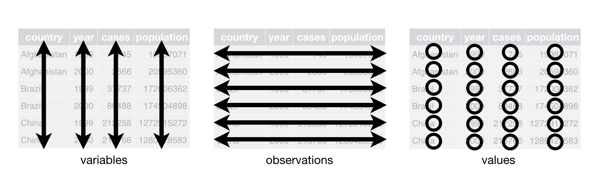
Figure 3.1: Tidy data graphic from http://r4ds.had.co.nz/tidy-data.html
Reading over this definition, you can begin to think about datasets that won’t follow this nice format. This format of data is also known as “long” format.
Learning check
(LC3.1) Give an example dataset that doesn’t follow this format.
- What features of this dataset might make it difficult to visualize?
- How could the dataset be tweaked to make it tidy?
(LC3.2) Say the following table are stock prices, how would you make this tidy?
| time | x | y | z |
|---|---|---|---|
| 2009-01-01 | 1.016 | -3.430 | 1.106 |
| 2009-01-02 | 1.095 | 1.726 | -3.154 |
| 2009-01-03 | -0.980 | 0.106 | -4.173 |
| 2009-01-04 | -1.274 | 0.915 | 0.243 |
| 2009-01-05 | -0.882 | 3.539 | 1.098 |
3.2 Datasets in the nycflights13 package
We likely have all flown on airplanes or know someone that has. Air travel has become an ever-present aspect of our daily lives. If you live in or are visiting a relatively large city and you walk around that city’s airport, you see gates showing flight information from many different airlines. And you will frequently see that some flights are delayed because of a variety of conditions. Are there ways that we can avoid having to deal with these flight delays?
We’d all like to arrive at our destinations on time whenever possible. (Unless you secretly love hanging out at airports. If you are one of these people, pretend for the moment that you are very much anticipating being at your final destination.) Throughout this book, we’re going to analyze data related to flights contained in the nycflights13 package we loaded earlier (Wickham 2017). Specifically, this package contains information about all flights that departed from NYC (e.g. EWR, JFK and LGA) in 2013 in 5 data sets:
flights: information on all 336,776 flightsweather: hourly meterological data for each airportplanes: construction information about each planeairports: airport names and locationsairlines: translation between two letter carrier codes and names
We will begin by loading in the flights dataset and getting an idea of its structure. Run the following in your console
data(flights)This line of code loads in the flights dataset that is stored in the nycflights13 package. This dataset and most others presented in this book will be in the “data frame” format in R. Data frames are essentially spreadsheets and allow us to look at collections of variables that are tightly coupled together.
The best way to get a feel for a data frame is to use the View function in RStudio. This command will be given throughout the book as a reminder, but the actual output will be hidden. Run View(flights) in R and look over this data frame. You should slowly get into the habit of always Viewing any data frames that come your way.
Learning check
(LC3.3) What does any ONE row in this flights dataset refer to?
- A. Data on an airline
- B. Data on a flight
- C. Data on an airport
- D. Data on multiple flights
By running View(flights), we see the different variables listed in the columns and we see that there are different types of variables. Some of the variables like distance, day, and arr_delay are what we will call quantitative variables. These variables vary in a numerical way. Other variables here are categorical.
Note that if you look in the leftmost column of the View(flights) output, you will see a column of numbers. These are the row numbers of the dataset. If you glance across a row with the same number, say row 5, you can get an idea of what each row corresponds to. In other words, this will allow you to identify what object is being referred to in a given row. This is often called the observational unit. The observational unit in this example is an individual flight departing New York City in 2013. You can identify the observational unit by determining what the thing is that is being measured in each of the variables.
Note: Frequently the first thing you should do when given a dataset is to
- identify the observational unit,
- specify the variables, and
- give the types of variables you are presented with.
The glimpse() command in the tibble package provides us with much of the above information and more:
glimpse(flights)## Observations: 336,776
## Variables: 19
## $ year <int> 2013, 2013, 2013, 2013, 2013, 2013, 2013, 20...
## $ month <int> 1, 1, 1, 1, 1, 1, 1, 1, 1, 1, 1, 1, 1, 1, 1,...
## $ day <int> 1, 1, 1, 1, 1, 1, 1, 1, 1, 1, 1, 1, 1, 1, 1,...
## $ dep_time <int> 517, 533, 542, 544, 554, 554, 555, 557, 557,...
## $ sched_dep_time <int> 515, 529, 540, 545, 600, 558, 600, 600, 600,...
## $ dep_delay <dbl> 2, 4, 2, -1, -6, -4, -5, -3, -3, -2, -2, -2,...
## $ arr_time <int> 830, 850, 923, 1004, 812, 740, 913, 709, 838...
## $ sched_arr_time <int> 819, 830, 850, 1022, 837, 728, 854, 723, 846...
## $ arr_delay <dbl> 11, 20, 33, -18, -25, 12, 19, -14, -8, 8, -2...
## $ carrier <chr> "UA", "UA", "AA", "B6", "DL", "UA", "B6", "E...
## $ flight <int> 1545, 1714, 1141, 725, 461, 1696, 507, 5708,...
## $ tailnum <chr> "N14228", "N24211", "N619AA", "N804JB", "N66...
## $ origin <chr> "EWR", "LGA", "JFK", "JFK", "LGA", "EWR", "E...
## $ dest <chr> "IAH", "IAH", "MIA", "BQN", "ATL", "ORD", "F...
## $ air_time <dbl> 227, 227, 160, 183, 116, 150, 158, 53, 140, ...
## $ distance <dbl> 1400, 1416, 1089, 1576, 762, 719, 1065, 229,...
## $ hour <dbl> 5, 5, 5, 5, 6, 5, 6, 6, 6, 6, 6, 6, 6, 6, 6,...
## $ minute <dbl> 15, 29, 40, 45, 0, 58, 0, 0, 0, 0, 0, 0, 0, ...
## $ time_hour <dttm> 2013-01-01 05:00:00, 2013-01-01 05:00:00, 2...Learning check
(LC3.4) What are some examples in this dataset of categorical variables? What makes them different than quantitative variables?
(LC3.5) What does int, num, and chr mean in the output above?
(LC3.6) How many different columns are in this dataset?
(LC3.7) How many different rows are in this dataset?
We see that glimpse will give you the first few entries of each variable in a row after the variable. In addition, the type of the variable is given immediately after each variable’s name inside < >. Here, int and num refer to quantitative variables. In contrast, chr refers to categorical variables. One more type of variable is given here with the time_hour variable: dttm. As you may suspect, this variable corresponds to a specific date and time of day.
Another nice feature of R is the help system. You can get help in R by simply entering a question mark before the name of a function or an object and you will be presented with a page showing the documentation. Since glimpse is a function defined in the tibble package, you can further emphasize that you’d like to look at the help for that specific glimpse function by adding the two columns between the package name and the function. Note that these output help files is omitted here but the flights help can be accessed here on page 3 of the PDF document.
?tibble::glimpse
?flights
Another aspect of tidy data is a description of what each variable in the dataset represents. This helps others to understand what your variable names mean and what they correspond to. If we look at the output of ?flights, we can see that a description of each variable by name is given.
An important feature to ALWAYS include with your data is the appropriate units of measurement. We’ll see this further when we work with the dep_delay variable in Chapter 4. (It’s in minutes, but you’d get some really strange interpretations if you thought it was in hours or seconds. UNITS MATTER!)
3.3 How is flights tidy?
We see that flights has a rectangular shape with each row corresponding to a different flight and each column corresponding to a characteristic of that flight. This matches exactly with how Hadley Wickham defined tidy data:
- Each variable forms a column.
- Each observation forms a row.
But what about the third property?
- Each type of observational unit forms a table.
We identified earlier that the observational unit in the flights dataset is an individual flight. And we have shown that this dataset consists of 336,776 flights with 19 variables. In other words, some rows of this dataset don’t refer to a measurement on an airline or on an airport. They specifically refer to characteristics/measurements on a given flight from New York City in 2013.
By contrast, also included in the nycflights13 package are datasets with different observational units (Wickham 2017):
weather: hourly meteorological data for each airportplanes: construction information about each planeairports: airport names and locationsairlines: translation between two letter carrier codes and names
You may have been asking yourself what carrier refers to in the glimpse(flights) output above. The airlines dataset provides a description of this with each airline being the observational unit:
data(airlines)
airlines
## # A tibble: 16 x 2
## carrier name
## <chr> <chr>
## 1 9E Endeavor Air Inc.
## 2 AA American Airlines Inc.
## 3 AS Alaska Airlines Inc.
## 4 B6 JetBlue Airways
## 5 DL Delta Air Lines Inc.
## 6 EV ExpressJet Airlines Inc.
## 7 F9 Frontier Airlines Inc.
## 8 FL AirTran Airways Corporation
## 9 HA Hawaiian Airlines Inc.
## 10 MQ Envoy Air
## 11 OO SkyWest Airlines Inc.
## 12 UA United Air Lines Inc.
## 13 US US Airways Inc.
## 14 VX Virgin America
## 15 WN Southwest Airlines Co.
## 16 YV Mesa Airlines Inc.As can be seen here when you just enter the name of an object in R, by default it will print the contents of that object to the screen. Be careful! It’s usually better to use the View() function in RStudio since larger objects may take awhile to print to the screen and it likely won’t be helpful to you to have hundreds of lines outputted.
Learning check
(LC3.8) Run the following block of code in RStudio to load and view each of the four data frames in the nycflights13 package. Switch between the different tabs that have opened to view each of the four data frames. Describe in two sentences for each data frame what stands out to you and what the most important features are of each.
data(weather)
data(planes)
data(airports)
data(airlines)
View(weather)
View(planes)
View(airports)
View(airlines)
3.3.1 Identification variables
There is a subtle difference between the kinds of variables that you will encounter in data frames. The airports data frame you worked with above contains data in these different kinds. Let’s pull them apart using the glimpse function:
glimpse(airports)## Observations: 1,458
## Variables: 8
## $ faa <chr> "04G", "06A", "06C", "06N", "09J", "0A9", "0G6", "0G7...
## $ name <chr> "Lansdowne Airport", "Moton Field Municipal Airport",...
## $ lat <dbl> 41.13047, 32.46057, 41.98934, 41.43191, 31.07447, 36....
## $ lon <dbl> -80.61958, -85.68003, -88.10124, -74.39156, -81.42778...
## $ alt <int> 1044, 264, 801, 523, 11, 1593, 730, 492, 1000, 108, 4...
## $ tz <dbl> -5, -6, -6, -5, -5, -5, -5, -5, -5, -8, -5, -6, -5, -...
## $ dst <chr> "A", "A", "A", "A", "A", "A", "A", "A", "U", "A", "A"...
## $ tzone <chr> "America/New_York", "America/Chicago", "America/Chica...The variables faa and name are what we will call identification variables. They are mainly used to provide a name to the observational unit. Here the observational unit is an airport and the faa gives the code provided by the FAA for that airport while the name variable gives the longer more natural name of the airport. These ID variables differ from the other variables that are often called measurement or characteristic variables. The remaining variables (aside from faa and name) are of this type in airports. They don’t uniquely identify the observational unit, but instead describe properties of the observational unit. For organizational purposes, it is best practice to have your identification variables in the far leftmost columns of your data frame.
Learning check
(LC3.9) What properties of the observational unit do each of lat, lon, alt, tz, dst, and tzone describe for the airports data frame?
(LC3.10) Provide the names of variables in a data frame with at least three variables in which one of them is an identification variable and the other two are not.
3.4 Normal forms of data
The datasets included in the nycflights13 package are in a form that minimizes redundancy of data. We will see that there are ways to merge (or join) the different tables together easily. We are capable of doing so because each of the tables have keys in common to relate one to another. This is an important property of normal forms of data. The process of decomposing data frames into less redundant tables without losing information is called normalization. More information is available on Wikipedia.
We saw an example of this above with the airlines dataset. While the flights data frame could also include a column with the names of the airlines instead of the carrier code, this would be repetitive since there is a unique mapping of the carrier code to the name of the airline/carrier.
Below an example is given showing how to join the airlines data frame together with the flights data frame by linking together the two datasets via a common key of "carrier". Note that this “joined” data frame is assigned to a new data frame called joined_flights. The key variable that we frequently join by is one of the identification variables mentioned above.
library(dplyr)
joined_flights <- inner_join(x = flights, y = airlines, by = "carrier")View(joined_flights)If we View this dataset, we see a new variable has been created called name. (We will see in Subsection 5.4.2 ways to change name to a more descriptive variable name.) More discussion about joining data frames together will be given in Chapter 5. We will see there that the names of the columns to be linked need not match as they did here with "carrier".
Learning check
(LC3.11) What are common characteristics of “tidy” datasets?
(LC3.12) What makes “tidy” datasets useful for organizing data?
(LC3.13) How many variables are presented in the table below? What does each row correspond to? (Hint: You may not be able to answer both of these questions immediately but take your best guess.)
| students | faculty |
|---|---|
| 4 | 2 |
| 6 | 3 |
(LC3.14) The confusion you may have encountered in Question 3 is a common one those that work with data are commonly presented with. This dataset is not tidy. Actually, the dataset in Question 4 has three variables not the two that were presented. Make a guess as to what these variables are and present a tidy dataset instead of this untidy one given in Question 4.
(LC3.15) The actual data presented in Question 4 is given below in tidy data format:
| role | Sociology? | Type of School |
|---|---|---|
| student | TRUE | Public |
| student | TRUE | Public |
| student | TRUE | Public |
| student | TRUE | Public |
| student | FALSE | Public |
| student | FALSE | Public |
| student | FALSE | Private |
| student | FALSE | Private |
| student | FALSE | Private |
| student | FALSE | Private |
| faculty | TRUE | Public |
| faculty | TRUE | Public |
| faculty | FALSE | Public |
| faculty | FALSE | Private |
| faculty | FALSE | Private |
- What does each row correspond to?
- What are the different variables in this data frame?
- The
Sociology?variable is known as a logical variable. What types of values does a logical variable take on?
(LC3.16) What are some advantages of data in normal forms? What are some disadvantages?
Review questions
Review questions have been designed using the fivethirtyeight R package (Ismay and Chunn 2017) with links to the corresponding FiveThirtyEight.com articles in our free DataCamp course Effective Data Storytelling using the tidyverse. The material in this chapter is covered in the Tidy Data chapter of the DataCamp course available here.
3.5 What’s to come?
In Chapter 4, we will further explore the distribution of a variable in a related dataset to flights: the temp variable in the weather dataset. We’ll be interested in understanding how this variable varies in relation to the values of other variables in the dataset. We will see that visualization is often a powerful tool in helping us see what is going on in a dataset. It will be a useful way to expand on the glimpse function we have seen here for tidy data.
References
Wickham, Hadley. 2014. “Tidy Data.” Journal of Statistical Software Volume 59 (Issue 10). https://www.jstatsoft.org/index.php/jss/article/view/v059i10/v59i10.pdf.
Wickham, Hadley. 2017. Nycflights13: Flights That Departed Nyc in 2013. https://CRAN.R-project.org/package=nycflights13.
Ismay, Chester, and Jennifer Chunn. 2017. Fivethirtyeight: Data and Code Behind the Stories and Interactives at ’Fivethirtyeight’. https://github.com/rudeboybert/fivethirtyeight.