Datasets and wrapper functions for tidyverse-friendly introductory linear regression, used in "Statistical Inference via Data Science: A ModernDive into R and the tidyverse" available at https://moderndive.com/.
Author
Maintainer: Albert Y. Kim albert.ys.kim@gmail.com (ORCID)
Authors:
Chester Ismay chester.ismay@gmail.com (ORCID)
Other contributors:
Andrew Bray abray@reed.edu (ORCID) [contributor]
Delaney Moran delaneyemoran@gmail.com [contributor]
Evgeni Chasnovski evgeni.chasnovski@gmail.com (ORCID) [contributor]
Will Hopper wjhopper510@gmail.com (ORCID) [contributor]
Benjamin S. Baumer ben.baumer@gmail.com (ORCID) [contributor]
Marium Tapal mariumtapal@gmail.com (ORCID) [contributor]
Wayne Ndlovu waynedndlovu5@gmail.com [contributor]
Catherine Peppers cpeppers@smith.edu [contributor]
Annah Mutaya annahmutaya18@gmail.com [contributor]
Anushree Goswami anushreeegoswami@gmail.com [contributor]
Ziyue Yang zyang2k@gmail.com (ORCID) [contributor]
Clara Li clarasepianli@gmail.com (ORCID) [contributor]
Caroline McKenna carolinemckenna101@gmail.com [contributor]
Catherine Park jcathyp@gmail.com (ORCID) [contributor]
Abbie Benfield abbidabbers@gmail.com [contributor]
Georgia Gans georgiagans@live.com [contributor]
Kacey Jean-Jacques kjeanjacques@smith.edu [contributor]
Swaha Bhattacharya itsswahabhattacharya@gmail.com [contributor]
Vivian Almaraz viviansofia101@gmail.com [contributor]
Elle Jo Whalen ewhalen@smith.edu [contributor]
Jacqueline Chen jchen76@smith.edu [contributor]
Michelle Flesaker mflesaker@smith.edu [contributor]
Irene Foster ifoster25@smith.edu [contributor]
Aushanae Haller aushanaenhaller@gmail.com [contributor]
Benjamin Bruncati kbruncati@smith.edu (ORCID) [contributor]
Quinn White quinnarlise@gmail.com (ORCID) [contributor]
Tianshu Zhang tzhang26@smith.edu (ORCID) [contributor]
Katelyn Diaz katndiaz@gmail.com (ORCID) [contributor]
Rose Porta rporta@smith.edu [contributor]
Renee Wu rwu30@smith.edu [contributor]
Arris Moise amoise@smith.edu [contributor]
Kate Phan kphan@smith.edu [contributor]
Grace Hartley grace.hartley@gmail.com [contributor]
Silas Weden silasweden@gmail.com [contributor]
Emma Vejcik evejcik@gmail.com [contributor]
Nikki Schuldt nikkischuldt@gmail.com [contributor]
Tess Goldmann tessgoldmann@aol.com [contributor]
Hongtong Lin cccynthialht@gmail.com [contributor]
Alejandra Munoz amunozgarcia@smith.edu [contributor]
Elina Gordon-Halpern egordonhalpern@smith.edu [contributor]
Haley Schmidt heschmidt00@gmail.com (ORCID) [contributor]
Examples
library(moderndive)

# Fit regression model:
life_exp_model <- lm(
  life_expectancy_2022 ~ gdp_per_capita,
  data = un_member_states_2024
)

# Regression tables:
get_regression_table(life_exp_model)
#> # A tibble: 2 × 7
#>   term           estimate std_error statistic p_value lower_ci upper_ci
#>   <chr>             <dbl>     <dbl>     <dbl>   <dbl>    <dbl>    <dbl>
#> 1 intercept          71.4     0.479    149.         0     70.5     72.4
#> 2 gdp_per_capita      0       0          9.85       0      0        0

# Information on each point in a regression:
get_regression_points(life_exp_model)
#> # A tibble: 188 × 5
#>       ID life_expectancy_2022 gdp_per_capita life_expectancy_2022_hat residual
#>    <int>                <dbl>          <dbl>                    <dbl>    <dbl>
#>  1     1                 53.6           356.                     71.5   -17.8
#>  2     2                 79.5          6810.                     72.3     7.17
#>  3     3                 78.0          4343.                     72.0     6.05
#>  4     4                 83.4         41993.                     76.9     6.49
#>  5     5                 62.1          3000.                     71.8    -9.69
#>  6     6                 77.8         19920.                     74.0     3.77
#>  7     7                 78.3         13651.                     73.2     5.11
#>  8     8                 76.1          7018.                     72.3     3.80
#>  9     9                 83.1         65100.                     80.0     3.13
#> 10    10                 82.3         52085.                     78.3     4.02
#> # ℹ 178 more rows

# Regression summaries
get_regression_summaries(life_exp_model)
#> # A tibble: 1 × 9
#>   r_squared adj_r_squared   mse  rmse sigma statistic p_value    df  nobs
#>       <dbl>         <dbl> <dbl> <dbl> <dbl>     <dbl>   <dbl> <dbl> <dbl>
#> 1     0.343         0.339  31.4  5.60  5.63      97.0       0     1   188

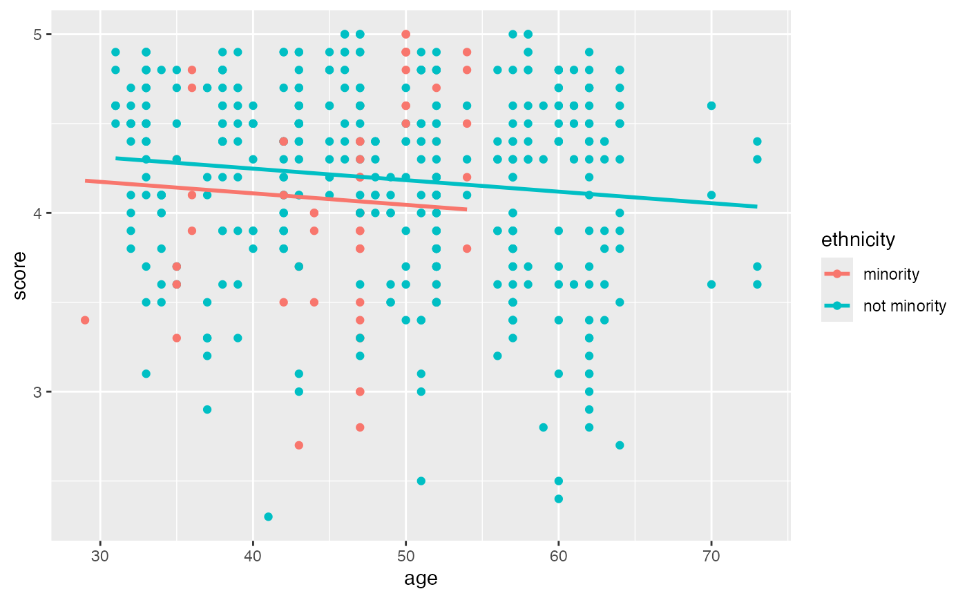
# Plotting parallel slopes models
library(ggplot2)
ggplot(evals, aes(x = age, y = score, color = ethnicity)) +
  geom_point() +
  geom_parallel_slopes(se = FALSE)