Take a `moderndive` into introductory linear regression with R

Summary

We present the moderndive R package of datasets and functions for tidyverse-friendly introductory linear regression (Wickham, Averick, et al. 2019). These tools leverage the well-developed tidyverse and broom packages to facilitate 1) working with regression tables that include confidence intervals, 2) accessing regression outputs on an observation level (e.g. fitted/predicted values and residuals), 3) inspecting scalar summaries of regression fit (e.g. $R^2$ , $R^2_{adj}$ , and mean squared error), and 4) visualizing parallel slopes regression models using ggplot2-like syntax (Wickham, Chang, et al. 2019; Robinson and Hayes 2019). This R package is designed to supplement the book “Statistical Inference via Data Science: A ModernDive into R and the Tidyverse” (Ismay and Kim 2019). Note that the book is also available online at https://moderndive.com and is referred to as “ModernDive” for short.

Statement of Need

Linear regression has long been a staple of introductory statistics courses. While the curricula of introductory statistics courses has much evolved of late, the overall importance of regression remains the same (American Statistical Association Undergraduate Guidelines Workgroup 2016). Furthermore, while the use of the R statistical programming language for statistical analysis is not new, recent developments such as the tidyverse suite of packages have made statistical computation with R accessible to a broader audience (Wickham, Averick, et al. 2019). We go one step further by leveraging the tidyverse and the broom packages to make linear regression accessible to students taking an introductory statistics course (Robinson and Hayes 2019). Such students are likely to be new to statistical computation with R; we designed moderndive with these students in mind.

Introduction

Let’s load all the R packages we are going to need.

library(moderndive)
library(ggplot2)
library(dplyr)
library(knitr)
library(broom)

Let’s consider data gathered from end of semester student evaluations for a sample of 463 courses taught by 94 professors from the University of Texas at Austin (Diez, Barr, and Çetinkaya-Rundel 2015). This data is included in the evals data frame from the moderndive package.

In the following table, we present a subset of 9 of the 14 variables included for a random sample of 5 courses¹:

ID uniquely identifies the course whereas prof_ID identifies the professor who taught this course. This distinction is important since many professors taught more than one course.
score is the outcome variable of interest: average professor evaluation score out of 5 as given by the students in this course.
The remaining variables are demographic variables describing that course’s instructor, including bty_avg (average “beauty” score) for that professor as given by a panel of 6 students.²

ID	prof_ID	score	age	bty_avg	gender	ethnicity	language	rank
129	23	3.7	62	3.000	male	not minority	english	tenured
109	19	4.7	46	4.333	female	not minority	english	tenured
28	6	4.8	62	5.500	male	not minority	english	tenured
434	88	2.8	62	2.000	male	not minority	english	tenured
330	66	4.0	64	2.333	male	not minority	english	tenured

Regression analysis the “good old-fashioned” way

Let’s fit a simple linear regression model of teaching score as a function of instructor age using the lm() function.

score_model <- lm(score ~ age, data = evals)

Let’s now study the output of the fitted model score_model “the good old-fashioned way”: using summary() which calls summary.lm() behind the scenes (we’ll refer to them interchangeably throughout this paper).

summary(score_model)
## 
## Call:
## lm(formula = score ~ age, data = evals)
## 
## Residuals:
##     Min      1Q  Median      3Q     Max 
## -1.9185 -0.3531  0.1172  0.4172  0.8825 
## 
## Coefficients:
##              Estimate Std. Error t value Pr(>|t|)    
## (Intercept)  4.461932   0.126778  35.195   <2e-16 ***
## age         -0.005938   0.002569  -2.311   0.0213 *  
## ---
## Signif. codes:  0 '***' 0.001 '**' 0.01 '*' 0.05 '.' 0.1 ' ' 1
## 
## Residual standard error: 0.5413 on 461 degrees of freedom
## Multiple R-squared:  0.01146,    Adjusted R-squared:  0.009311 
## F-statistic: 5.342 on 1 and 461 DF,  p-value: 0.02125

Regression analysis using `moderndive`

As an improvement to base R’s regression functions, we’ve included three functions in the moderndive package that take a fitted model object as input and return the same information as summary.lm(), but output them in tidyverse-friendly format (Wickham, Averick, et al. 2019). As we’ll see later, while these three functions are thin wrappers to existing functions in the broom package for converting statistical objects into tidy tibbles, we modified them with the introductory statistics student in mind (Robinson and Hayes 2019).

Get a tidy regression table with confidence intervals:

get_regression_table(score_model)
## # A tibble: 2 × 7
##   term      estimate std_error statistic p_value lower_ci upper_ci
##   <chr>        <dbl>     <dbl>     <dbl>   <dbl>    <dbl>    <dbl>
## 1 intercept    4.46      0.127     35.2    0        4.21     4.71 
## 2 age         -0.006     0.003     -2.31   0.021   -0.011   -0.001

Get information on each point/observation in your regression, including fitted/predicted values and residuals, in a single data frame:

get_regression_points(score_model)
## # A tibble: 463 × 5
##       ID score   age score_hat residual
##    <int> <dbl> <int>     <dbl>    <dbl>
##  1     1   4.7    36      4.25    0.452
##  2     2   4.1    36      4.25   -0.148
##  3     3   3.9    36      4.25   -0.348
##  4     4   4.8    36      4.25    0.552
##  5     5   4.6    59      4.11    0.488
##  6     6   4.3    59      4.11    0.188
##  7     7   2.8    59      4.11   -1.31 
##  8     8   4.1    51      4.16   -0.059
##  9     9   3.4    51      4.16   -0.759
## 10    10   4.5    40      4.22    0.276
## # ℹ 453 more rows

Get scalar summaries of a regression fit including $R^2$ and $R^2_{adj}$ but also the (root) mean-squared error:

get_regression_summaries(score_model)
## # A tibble: 1 × 9
##   r_squared adj_r_squared   mse  rmse sigma statistic p_value    df
##       <dbl>         <dbl> <dbl> <dbl> <dbl>     <dbl>   <dbl> <dbl>
## 1     0.011         0.009 0.292 0.540 0.541      5.34   0.021     1
## # ℹ 1 more variable: nobs <dbl>

Furthermore, say you would like to create a visualization of the relationship between two numerical variables and a third categorical variable with $k$ levels. Let’s create this using a colored scatterplot via the ggplot2 package for data visualization (Wickham, Chang, et al. 2019). Using geom_smooth(method = "lm", se = FALSE) yields a visualization of an interaction model where each of the $k$ regression lines has their own intercept and slope. For example in , we extend our previous regression model by now mapping the categorical variable ethnicity to the color aesthetic.

# Code to visualize interaction model:
ggplot(evals, aes(x = age, y = score, color = ethnicity)) +
  geom_point() +
  geom_smooth(method = "lm", se = FALSE) +
  labs(x = "Age", y = "Teaching score", color = "Ethnicity")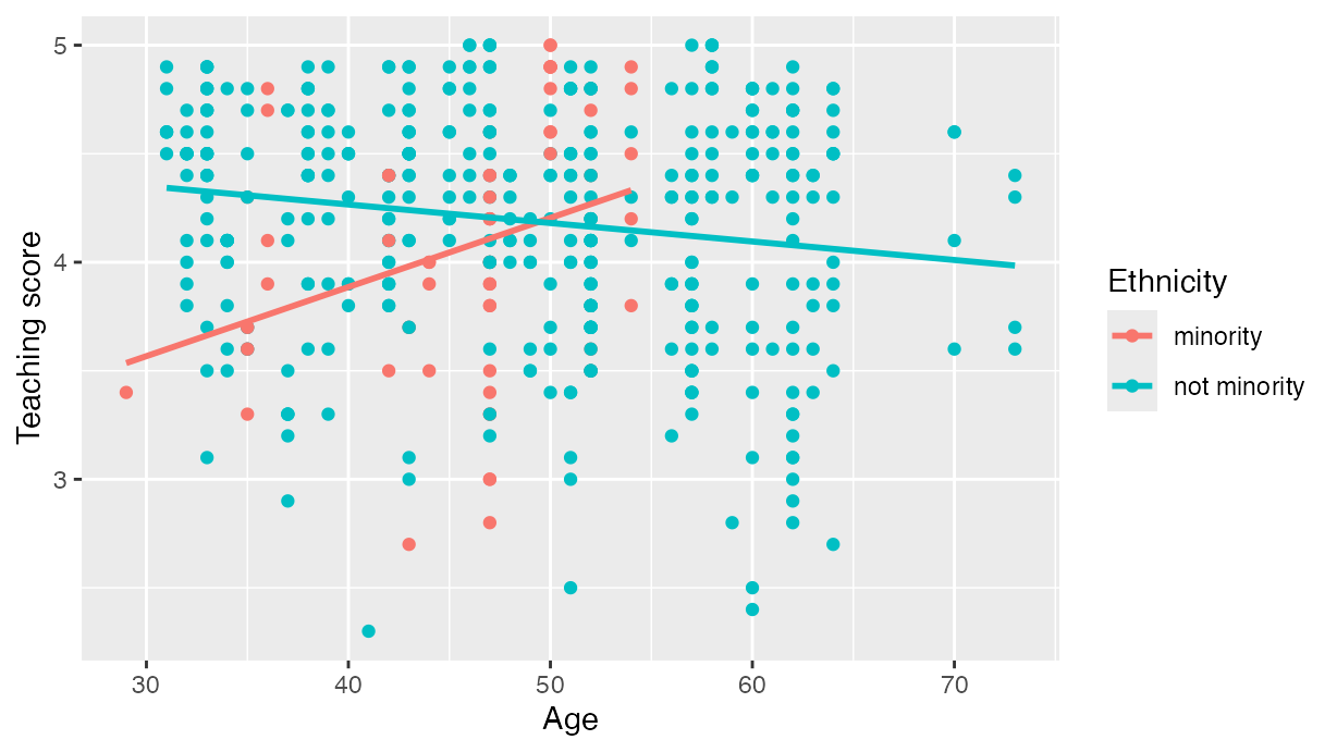

Visualization of interaction model.

However, many introductory statistics courses start with the easier to teach “common slope, different intercepts” regression model, also known as the parallel slopes model. However, no argument to plot such models exists within geom_smooth().

Evgeni Chasnovski thus wrote a custom geom_ extension to ggplot2 called geom_parallel_slopes(); this extension is included in the moderndive package. Much like geom_smooth() from the ggplot2 package, you add geom_parallel_slopes() as a layer to the code, resulting in .

# Code to visualize parallel slopes model:
ggplot(evals, aes(x = age, y = score, color = ethnicity)) +
  geom_point() +
  geom_parallel_slopes(se = FALSE) +
  labs(x = "Age", y = "Teaching score", color = "Ethnicity")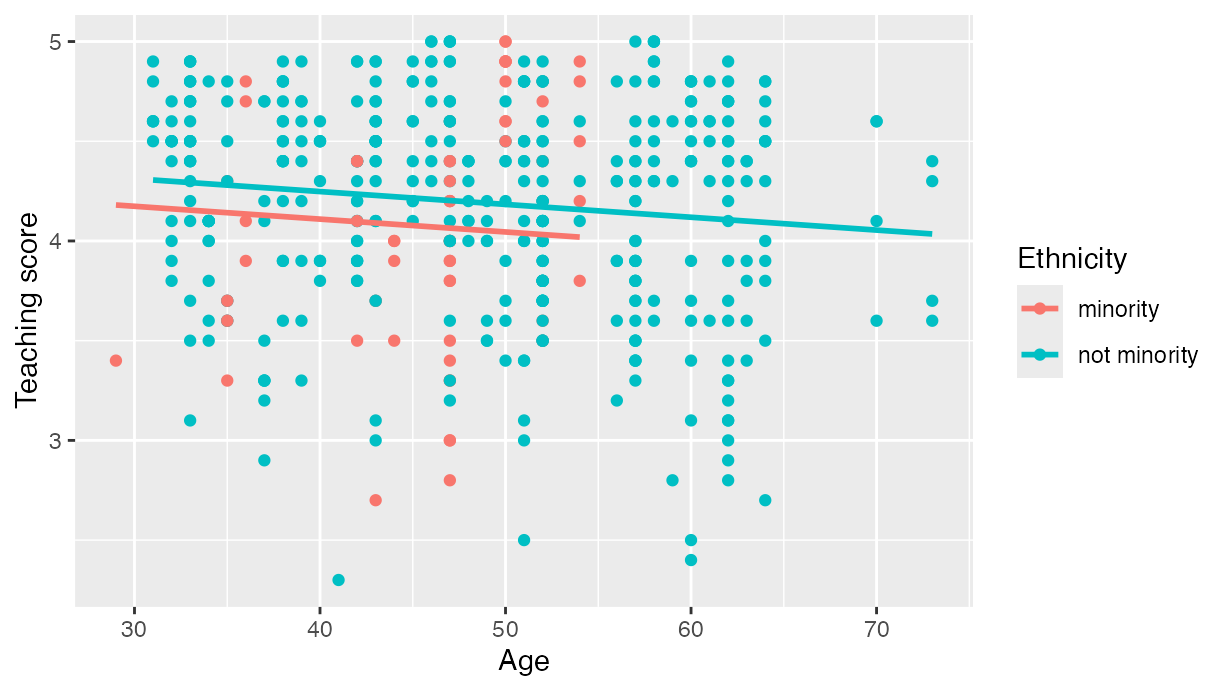

Visualization of parallel slopes model.

Repository README

In the GitHub repository README, we present an in-depth discussion of six features of the moderndive package:

Focus less on p-value stars, more confidence intervals
Outputs as tibbles
Produce residual analysis plots from scratch using ggplot2
A quick-and-easy Kaggle predictive modeling competition submission!
Visual model selection: plot parallel slopes & interaction regression models
Produce metrics on the quality of regression model fits

Furthermore, we discuss the inner-workings of the moderndive package:

It leverages the broom package in its wrappers
It builds a custom ggplot2 geometry for the geom_parallel_slopes() function that allows for quick visualization of parallel slopes models in regression.

Author contributions

Albert Y. Kim and Chester Ismay contributed equally to the development of the moderndive package. Albert Y. Kim wrote a majority of the initial version of this manuscript with Chester Ismay writing the rest. Max Kuhn provided guidance and feedback at various stages of the package development and manuscript writing.

Acknowledgments

Many thanks to Jenny Smetzer @smetzer180, Luke W. Johnston @lwjohnst86, and Lisa Rosenthal @lisamr for their helpful feedback for this paper and to Evgeni Chasnovski @echasnovski for contributing the geom_parallel_slopes() function via GitHub pull request. The authors do not have any financial support to disclose.

References

American Statistical Association Undergraduate Guidelines Workgroup. 2016. “‘Guidelines for Assessment and Instruction in Statistics Education (GAISE) in Statistics Education (GAISE) College Report College Report 2016’.” Alexandria, VA: American Statistical Association.

Diez, D. M., C. D. Barr, and M. Çetinkaya-Rundel. 2015. OpenIntro Statistics. OpenIntro, Incorporated. https://doi.org/10.5070/T573020084.

Ismay, Chester., and Albert Y. Kim. 2019. Statistical Inference via Data Science: A ModernDive into r and the Tidyverse. Chapman & Hall/CRC the r Series. CRC Press. https://doi.org/10.1080/00224065.2020.1848366.

Robinson, David, and Alex Hayes. 2019. Broom: Convert Statistical Analysis Objects into Tidy Tibbles. https://CRAN.R-project.org/package=broom.

Wickham, Hadley, Mara Averick, Jennifer Bryan, Winston Chang, Lucy D’Agostino McGowan, Romain François, Garrett Grolemund, et al. 2019. “Welcome to the tidyverse.” Journal of Open Source Software 4 (43): 1686. https://doi.org/10.21105/joss.01686.

Wickham, Hadley, Winston Chang, Lionel Henry, Thomas Lin Pedersen, Kohske Takahashi, Claus Wilke, Kara Woo, and Hiroaki Yutani. 2019. ggplot2: Create Elegant Data Visualisations Using the Grammar of Graphics. https://doi.org/10.1007/978-0-387-98141-3.

Albert Y. Kim, Chester Ismay, and Max Kuhn

2025-10-26

Summary

Statement of Need

Introduction

Regression analysis the “good old-fashioned” way

Regression analysis using `moderndive`

Repository README

Author contributions

Acknowledgments

References

Take a `moderndive` into introductory linear regression with R

Albert Y. Kim, Chester Ismay, and Max Kuhn

2025-10-26

Summary

Statement of Need

Introduction

Regression analysis the “good old-fashioned” way

Regression analysis using moderndive

Repository README

Author contributions

Acknowledgments

References

Regression analysis using `moderndive`