Tidyverse-Friendly Introductory Linear Regression • moderndive

moderndive R Package

Overview

The moderndive R package consists of datasets and functions for tidyverse-friendly introductory linear regression. These tools leverage the well-developed tidyverse and broom packages to facilitate

Working with regression tables that include confidence intervals
Accessing regression outputs on an observation level (e.g. fitted/predicted values and residuals)
Inspecting scalar summaries of regression fit (e.g. R-squared, R-squared adjusted, and mean squared error)
Visualizing parallel slopes regression models using ggplot2-like syntax.

This R package is designed to supplement the book “Statistical Inference via Data Science: A ModernDive into R and the Tidyverse” available at ModernDive.com. For more background, read our Journal of Open Source Education paper.

Installation

Get the released version from CRAN:

install.packages("moderndive")

Or the development version from GitHub:

# If you haven't installed remotes yet, do so:
# install.packages("remotes")
remotes::install_github("moderndive/moderndive")

Basic usage

library(moderndive)
score_model <- lm(score ~ age, data = evals)

Get a tidy regression table with confidence intervals:

get_regression_table(score_model)

## # A tibble: 2 × 7
##   term      estimate std_error statistic p_value lower_ci upper_ci
##   <chr>        <dbl>     <dbl>     <dbl>   <dbl>    <dbl>    <dbl>
## 1 intercept    4.46      0.127     35.2    0        4.21     4.71 
## 2 age         -0.006     0.003     -2.31   0.021   -0.011   -0.001

Get information on each point/observation in your regression, including fitted/predicted values and residuals, in a single data frame:

get_regression_points(score_model)

## # A tibble: 463 × 5
##       ID score   age score_hat residual
##    <int> <dbl> <int>     <dbl>    <dbl>
##  1     1   4.7    36      4.25    0.452
##  2     2   4.1    36      4.25   -0.148
##  3     3   3.9    36      4.25   -0.348
##  4     4   4.8    36      4.25    0.552
##  5     5   4.6    59      4.11    0.488
##  6     6   4.3    59      4.11    0.188
##  7     7   2.8    59      4.11   -1.31 
##  8     8   4.1    51      4.16   -0.059
##  9     9   3.4    51      4.16   -0.759
## 10    10   4.5    40      4.22    0.276
## # … with 453 more rows

Get scalar summaries of a regression fit including R-squared and R-squared adjusted but also the (root) mean-squared error:

get_regression_summaries(score_model)

## # A tibble: 1 × 9
##   r_squared adj_r_squared   mse  rmse sigma statistic p_value    df  nobs
##       <dbl>         <dbl> <dbl> <dbl> <dbl>     <dbl>   <dbl> <dbl> <dbl>
## 1     0.011         0.009 0.292 0.540 0.541      5.34   0.021     1   463

Visualize parallel slopes models using the geom_parallel_slopes() custom ggplot2 geometry:

library(ggplot2)
ggplot(evals, aes(x = age, y = score, color = ethnicity)) +
  geom_point() +
  geom_parallel_slopes(se = FALSE) +
  labs(x = "Age", y = "Teaching score", color = "Ethnicity")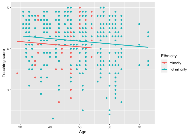

Statement of Need

Linear regression has long been a staple of introductory statistics courses. While the curricula of introductory statistics courses has much evolved of late, the overall importance of regression remains the same. Furthermore, while the use of the R statistical programming language for statistical analysis is not new, recent developments such as the tidyverse suite of packages have made statistical computation with R accessible to a broader audience. We go one step further by leveraging the tidyverse and the broom packages to make linear regression accessible to students taking an introductory statistics course. Such students are likely to be new to statistical computation with R; we designed moderndive with these students in mind.

Contributor code of conduct

Please note that this project is released with a Contributor Code of Conduct. By participating in this project you agree to abide by its terms.

Six features

Why should you use the moderndive package for introductory linear regression? Here are six features:

Focus less on p-value stars, more confidence intervals
Outputs as tibbles
Produce residual analysis plots from scratch using ggplot2
A quick-and-easy Kaggle predictive modeling competition submission!
Visual model selection: plot parallel slopes & interaction regression models
Produce metrics on the quality of regression model fits

Data background

We first discuss the model and data background. The data consists of end of semester student evaluations for a sample of 463 courses taught by 94 professors from the University of Texas at Austin. This data is included in the evals data frame from the moderndive package.

In the following table, we present a subset of 9 of the 14 variables included for a random sample of 5 courses[1]:

ID uniquely identifies the course whereas prof_ID identifies the professor who taught this course. This distinction is important since many professors taught more than one course.
score is the outcome variable of interest: average professor evaluation score out of 5 as given by the students in this course.
The remaining variables are demographic variables describing that course’s instructor, including bty_avg (average “beauty” score) for that professor as given by a panel of 6 students.[2]

ID	prof_ID	score	age	bty_avg	gender	ethnicity	language	rank
355	71	4.9	50	3.333	male	minority	english	teaching
262	49	4.3	52	3.167	male	not minority	english	tenured
441	89	3.7	35	7.833	female	minority	english	tenure track
51	10	4.3	47	5.500	male	not minority	english	teaching
49	9	4.5	33	4.667	female	not minority	english	tenure track

1. Focus less on p-value stars, more confidence intervals

We argue that the summary.lm() output is deficient in an introductory statistics setting because:

The Signif. codes: 0 '' 0.001 '**' 0.01 '*' 0.05 '.' 0.1 ' ' 1 only encourage p-hacking. In case you have not yet been convinced of the perniciousness of p-hacking, perhaps comedian John Oliver can convince you.
While not a silver bullet for eliminating misinterpretations of statistical inference, confidence intervals present students with a sense of the associated effect sizes of any explanatory variables. Thus, practical as well as statistical significance is emphasized. These are not included by default in the output of summary.lm().

Instead of summary(), let’s use the get_regression_table() function:

get_regression_table(score_model)

## # A tibble: 2 × 7
##   term      estimate std_error statistic p_value lower_ci upper_ci
##   <chr>        <dbl>     <dbl>     <dbl>   <dbl>    <dbl>    <dbl>
## 1 intercept    4.46      0.127     35.2    0        4.21     4.71 
## 2 age         -0.006     0.003     -2.31   0.021   -0.011   -0.001

Observe how the p-value stars are omitted and confidence intervals for the point estimates of all regression parameters are included by default. By including them in the output, we can then emphasize to students that they “surround” the point estimates in the estimate column. Note the confidence level is defaulted to 95%; this default can be changed using the conf.level argument:

get_regression_table(score_model, conf.level = 0.99)

## # A tibble: 2 × 7
##   term      estimate std_error statistic p_value lower_ci upper_ci
##   <chr>        <dbl>     <dbl>     <dbl>   <dbl>    <dbl>    <dbl>
## 1 intercept    4.46      0.127     35.2    0        4.13     4.79 
## 2 age         -0.006     0.003     -2.31   0.021   -0.013    0.001

2. Outputs as tibbles

While one might argue that extracting the intercept and slope coefficients can be “simply” done using coefficients(score_model), what about the standard errors? For example, a Google query of “how do I extract standard errors from lm in R” yielded results from the R mailing list and from Cross Validated suggesting we run:

sqrt(diag(vcov(score_model)))

## (Intercept)         age 
## 0.126778499 0.002569157

We argue that this task shouldn’t be this hard, especially in an introductory statistics setting. To rectify this, the three get_regression_* functions all return data frames in the tidyverse-style tibble (tidy table) format. Therefore you can extract columns using the pull() function from the dplyr package:

library(dplyr)
get_regression_table(score_model) %>%
  pull(std_error)

## [1] 0.127 0.003

or equivalently you can use the $ sign operator from base R:

get_regression_table(score_model)$std_error

## [1] 0.127 0.003

Furthermore, by piping the above get_regression_table(score_model) output into the kable() function from the knitr package, you can obtain aesthetically pleasing regression tables in R Markdown documents, instead of tables written in jarring computer output font:

library(knitr)
get_regression_table(score_model) %>%
  kable()

term	estimate	std_error	statistic	p_value	lower_ci	upper_ci
intercept	4.462	0.127	35.195	0.000	4.213	4.711
age	-0.006	0.003	-2.311	0.021	-0.011	-0.001

3. Produce residual analysis plots from scratch using `ggplot2`

How can we extract point-by-point information from a regression model, such as the fitted/predicted values and the residuals? (Note we only display the first 10 out of 463 of such values for brevity’s sake.)

fitted(score_model)

##        1        2        3        4        5        6        7        8 
## 4.248156 4.248156 4.248156 4.248156 4.111577 4.111577 4.111577 4.159083 
##        9       10 
## 4.159083 4.224403

residuals(score_model)

##           1           2           3           4           5           6 
##  0.45184376 -0.14815624 -0.34815624  0.55184376  0.48842294  0.18842294 
##           7           8           9          10 
## -1.31157706 -0.05908286 -0.75908286  0.27559666

But why have the original explanatory/predictor age and outcome variable score in evals, the fitted/predicted values score_hat, and residual floating around in separate vectors? Since each observation relates to the same course, we argue it makes more sense to organize them together in the same data frame using get_regression_points():

score_model_points <- get_regression_points(score_model)
score_model_points

## # A tibble: 10 × 5
##       ID score   age score_hat residual
##    <int> <dbl> <int>     <dbl>    <dbl>
##  1     1   4.7    36      4.25    0.452
##  2     2   4.1    36      4.25   -0.148
##  3     3   3.9    36      4.25   -0.348
##  4     4   4.8    36      4.25    0.552
##  5     5   4.6    59      4.11    0.488
##  6     6   4.3    59      4.11    0.188
##  7     7   2.8    59      4.11   -1.31 
##  8     8   4.1    51      4.16   -0.059
##  9     9   3.4    51      4.16   -0.759
## 10    10   4.5    40      4.22    0.276

Observe that the original outcome variable score and explanatory/predictor variable age are now supplemented with the fitted/predicted values score_hat and residual columns. By putting the fitted values, predicted values, and residuals next to the original data, we argue that the computation of these values is less opaque. For example, instructors can emphasize how all values in the first row of output are computed.

Furthermore, recall that since all outputs in the moderndive package are tibble data frames, custom residual analysis plots can be created instead of relying on the default plots yielded by plot.lm(). For example, we can check for the normality of residuals using the histogram of residuals shown in .

# Code to visualize distribution of residuals:
ggplot(score_model_points, aes(x = residual)) +
  geom_histogram(bins = 20) +
  labs(x = "Residual", y = "Count")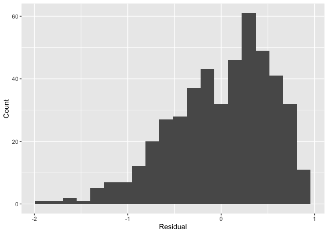

Histogram visualizing distribution of residuals.

As another example, we can investigate potential relationships between the residuals and all explanatory/predictor variables and the presence of heteroskedasticity using partial residual plots, like the partial residual plot over age shown in . If the term “heteroskedasticity” is new to you, it corresponds to the variability of one variable being unequal across the range of values of another variable. The presence of heteroskedasticity violates one of the assumptions of inference for linear regression.

# Code to visualize partial residual plot over age:
ggplot(score_model_points, aes(x = age, y = residual)) +
  geom_point() +
  labs(x = "Age", y = "Residual")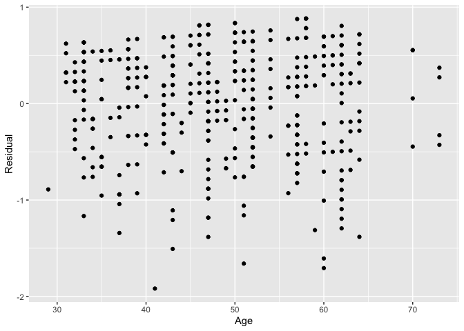

Partial residual residual plot over age.

4. A quick-and-easy Kaggle predictive modeling competition submission!

With the fields of machine learning and artificial intelligence gaining prominence, the importance of predictive modeling cannot be understated. Therefore, we’ve designed the get_regression_points() function to allow for a newdata argument to quickly apply a previously fitted model to new observations.

Let’s create an artificial “new” dataset consisting of two instructors of age 39 and 42 and save it in a tibble data frame called new_prof. We then set the newdata argument to get_regression_points() to apply our previously fitted model score_model to this new data, where score_hat holds the corresponding fitted/predicted values.

new_prof <- tibble(age = c(39, 42))
get_regression_points(score_model, newdata = new_prof)

## # A tibble: 2 × 3
##      ID   age score_hat
##   <int> <dbl>     <dbl>
## 1     1    39      4.23
## 2     2    42      4.21

Let’s do another example, this time using the Kaggle House Prices: Advanced Regression Techniques practice competition ( displays the homepage for this competition).

House prices Kaggle competition homepage.

This Kaggle competition requires you to fit/train a model to the provided train.csv training set to make predictions of house prices in the provided test.csv test set. We present an application of the get_regression_points() function allowing students to participate in this Kaggle competition. It will:

Read in the training and test data.
Fit a naive model of house sale price as a function of year sold to the training data.
Make predictions on the test data and write them to a submission.csv file that can be submitted to Kaggle using get_regression_points(). Note the use of the ID argument to use the id variable in test to identify the rows (a requirement of Kaggle competition submissions).

library(readr)
library(dplyr)
library(moderndive)

# Load in training and test set
train <- read_csv("https://moderndive.com/data/train.csv")
test <- read_csv("https://moderndive.com/data/test.csv")

# Fit model:
house_model <- lm(SalePrice ~ YrSold, data = train)

# Make predictions and save in appropriate data frame format:
submission <- house_model %>%
  get_regression_points(newdata = test, ID = "Id") %>%
  select(Id, SalePrice = SalePrice_hat)

# Write predictions to csv:
write_csv(submission, "submission.csv")

After submitting submission.csv to the leaderboard for this Kaggle competition, we obtain a “root mean squared logarithmic error” (RMSLE) score of 0.42918 as seen in .

Resulting Kaggle RMSLE score.

5. Visual model selection: plot parallel slopes & interaction regression models

For example, recall the earlier visualizations of the interaction and parallel slopes models for teaching score as a function of age and ethnicity we saw in Figures and . Let’s present both visualizations side-by-side in .

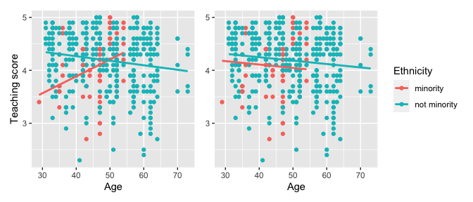
Interaction (left) and parallel slopes (right) models.

Students might be wondering “Why would you use the parallel slopes model on the right when the data clearly form an”X” pattern as seen in the interaction model on the left?” This is an excellent opportunity to gently introduce the notion of model selection and Occam’s Razor: an interaction model should only be used over a parallel slopes model if the additional complexity of the interaction model is warranted. Here, we define model “complexity/simplicity” in terms of the number of parameters in the corresponding regression tables:

# Regression table for interaction model:
interaction_evals <- lm(score ~ age * ethnicity, data = evals)
get_regression_table(interaction_evals)

## # A tibble: 4 × 7
##   term                    estimate std_error statistic p_value lower_ci upper_ci
##   <chr>                      <dbl>     <dbl>     <dbl>   <dbl>    <dbl>    <dbl>
## 1 intercept                  2.61      0.518      5.04   0        1.59     3.63 
## 2 age                        0.032     0.011      2.84   0.005    0.01     0.054
## 3 ethnicity: not minority    2.00      0.534      3.74   0        0.945    3.04 
## 4 age:ethnicitynot minor…   -0.04      0.012     -3.51   0       -0.063   -0.018

# Regression table for parallel slopes model:
parallel_slopes_evals <- lm(score ~ age + ethnicity, data = evals)
get_regression_table(parallel_slopes_evals)

## # A tibble: 3 × 7
##   term                    estimate std_error statistic p_value lower_ci upper_ci
##   <chr>                      <dbl>     <dbl>     <dbl>   <dbl>    <dbl>    <dbl>
## 1 intercept                  4.37      0.136     32.1    0        4.1      4.63 
## 2 age                       -0.006     0.003     -2.5    0.013   -0.012   -0.001
## 3 ethnicity: not minority    0.138     0.073      1.89   0.059   -0.005    0.282

The interaction model is “more complex” as evidenced by its regression table involving 4 rows of parameter estimates whereas the parallel slopes model is “simpler” as evidenced by its regression table involving only 3 parameter estimates. It can be argued however that this additional complexity is warranted given the clearly different slopes in the left-hand plot of .

We now present a contrasting example, this time from Chapter 6 of the online version of ModernDive Subsection 6.3.1 involving Massachusetts USA public high schools.[3] Let’s plot both the interaction and parallel slopes models in .

# Code to plot interaction and parallel slopes models for MA_schools
ggplot(
  MA_schools,
  aes(x = perc_disadvan, y = average_sat_math, color = size)
) +
  geom_point(alpha = 0.25) +
  labs(
    x = "% economically disadvantaged",
    y = "Math SAT Score",
    color = "School size"
  ) +
  geom_smooth(method = "lm", se = FALSE)

ggplot(
  MA_schools,
  aes(x = perc_disadvan, y = average_sat_math, color = size)
) +
  geom_point(alpha = 0.25) +
  labs(
    x = "% economically disadvantaged",
    y = "Math SAT Score",
    color = "School size"
  ) +
  geom_parallel_slopes(se = FALSE)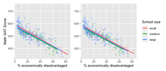

Interaction (left) and parallel slopes (right) models.

In terms of the corresponding regression tables, observe that the corresponding regression table for the parallel slopes model has 4 rows as opposed to the 6 for the interaction model, reflecting its higher degree of “model simplicity.”

# Regression table for interaction model:
interaction_MA <-
  lm(average_sat_math ~ perc_disadvan * size, data = MA_schools)
get_regression_table(interaction_MA)

## # A tibble: 6 × 7
##   term                    estimate std_error statistic p_value lower_ci upper_ci
##   <chr>                      <dbl>     <dbl>     <dbl>   <dbl>    <dbl>    <dbl>
## 1 intercept                594.       13.3      44.7     0      568.     620.   
## 2 perc_disadvan             -2.93      0.294    -9.96    0       -3.51    -2.35 
## 3 size: medium             -17.8      15.8      -1.12    0.263  -48.9     13.4  
## 4 size: large              -13.3      13.8      -0.962   0.337  -40.5     13.9  
## 5 perc_disadvan:sizemedi…    0.146     0.371     0.393   0.694   -0.585    0.877
## 6 perc_disadvan:sizelarge    0.189     0.323     0.586   0.559   -0.446    0.824

# Regression table for parallel slopes model:
parallel_slopes_MA <-
  lm(average_sat_math ~ perc_disadvan + size, data = MA_schools)
get_regression_table(parallel_slopes_MA)

## # A tibble: 4 × 7
##   term          estimate std_error statistic p_value lower_ci upper_ci
##   <chr>            <dbl>     <dbl>     <dbl>   <dbl>    <dbl>    <dbl>
## 1 intercept       588.       7.61     77.3     0       573.     603.  
## 2 perc_disadvan    -2.78     0.106   -26.1     0        -2.99    -2.57
## 3 size: medium    -11.9      7.54     -1.58    0.115   -26.7      2.91
## 4 size: large      -6.36     6.92     -0.919   0.359   -20.0      7.26

Unlike our earlier comparison of interaction and parallel slopes models in , in this case it could be argued that the additional complexity of the interaction model is not warranted since the 3 three regression lines in the left-hand interaction are already somewhat parallel. Therefore the simpler parallel slopes model should be favored.

Going one step further, notice how the three regression lines in the visualization of the parallel slopes model in the right-hand plot of have similar intercepts. In can thus be argued that the additional model complexity induced by introducing the categorical variable school size is not warranted. Therefore, a simple linear regression model using only perc_disadvan percent of the student body that are economically disadvantaged should be favored.

While many students will inevitably find these results depressing, in our opinion, it is important to additionally emphasize that such regression analyses can be used as an empowering tool to bring to light inequities in access to education and inform policy decisions.

6. Produce metrics on the quality of regression model fits

Recall the output of the standard summary.lm() from earlier:

## 
## Call:
## lm(formula = score ~ age, data = evals)
## 
## Residuals:
##     Min      1Q  Median      3Q     Max 
## -1.9185 -0.3531  0.1172  0.4172  0.8825 
## 
## Coefficients:
##              Estimate Std. Error t value Pr(>|t|)    
## (Intercept)  4.461932   0.126778  35.195   <2e-16 ***
## age         -0.005938   0.002569  -2.311   0.0213 *  
## ---
## Signif. codes:  0 '***' 0.001 '**' 0.01 '*' 0.05 '.' 0.1 ' ' 1
## 
## Residual standard error: 0.5413 on 461 degrees of freedom
## Multiple R-squared:  0.01146,    Adjusted R-squared:  0.009311 
## F-statistic: 5.342 on 1 and 461 DF,  p-value: 0.02125

Say we wanted to extract the scalar model summaries at the bottom of this output, such as R-squared, R-squared adjusted, the F-statistic, and the degrees of freedom df. We can do so using the get_regression_summaries() function.

get_regression_summaries(score_model)

## # A tibble: 1 × 9
##   r_squared adj_r_squared   mse  rmse sigma statistic p_value    df  nobs
##       <dbl>         <dbl> <dbl> <dbl> <dbl>     <dbl>   <dbl> <dbl> <dbl>
## 1     0.011         0.009 0.292 0.540 0.541      5.34   0.021     1   463

We’ve supplemented the standard scalar summaries output yielded by summary() with the mean squared error mse and root mean squared error rmse given their popularity in machine learning settings.

The inner workings

How does this all work? Let’s open the hood of the moderndive package.

Three wrappers to `broom` functions

As we mentioned earlier, the three get_regression_* functions are wrappers of functions from the broom package for converting statistical analysis objects into tidy tibbles along with a few added tweaks, but with the introductory statistics student in mind:

get_regression_table() is a wrapper for broom::tidy().
get_regression_points() is a wrapper for broom::augment().
get_regression_summaries is a wrapper for broom::glance().

Why did we take this approach to address the initial 5 common student questions at the outset of the article?

By writing wrappers to pre-existing functions, instead of creating new custom functions, there is minimal re-inventing of the wheel necessary.
In our experience, novice R users had a hard time understanding the broom package function names tidy(), augment(), and glance(). To make them more user-friendly, the moderndive package wrappers have much more intuitively named get_regression_table(), get_regression_points(), and get_regression_summaries().
The variables included in the outputs of the above 3 broom functions are not all applicable to an introductory statistics students and of those that were, we found they were not intuitive for new R users. We therefore cut out some of the variables from the output and renamed some of the remaining variables. For example, compare the outputs of the get_regression_points() wrapper function and the parent broom::augment() function.

get_regression_points(score_model)
broom::augment(score_model)

The source code for these three get_regression_* functions can be found on here.

Custom geometries

The geom_parallel_slopes() is a custom built geom extension to the ggplot2 package. For example, the ggplot2 webpage page gives instructions on how to create such extensions. The source code for geom_parallel_slopes() written by Evgeni Chasnovski can be found on GitHub.

For details on the remaining 5 variables, see the help file by running ?evals.
Note that gender was collected as a binary variable at the time of the study (2005).
For more details on this dataset, see the help file by running ?MA_schools.

moderndive R Package

Overview

Installation

Basic usage

Statement of Need

Contributor code of conduct

Six features

Data background

1. Focus less on p-value stars, more confidence intervals

2. Outputs as tibbles

3. Produce residual analysis plots from scratch using `ggplot2`

4. A quick-and-easy Kaggle predictive modeling competition submission!

5. Visual model selection: plot parallel slopes & interaction regression models

6. Produce metrics on the quality of regression model fits

The inner workings

Three wrappers to `broom` functions

Custom geometries

Links

License

Community

Citation

Developers

Dev status

moderndive R Package

Overview

Installation

Basic usage

Statement of Need

Contributor code of conduct

Six features

Data background

1. Focus less on p-value stars, more confidence intervals

2. Outputs as tibbles

3. Produce residual analysis plots from scratch using ggplot2

4. A quick-and-easy Kaggle predictive modeling competition submission!

5. Visual model selection: plot parallel slopes & interaction regression models

6. Produce metrics on the quality of regression model fits

The inner workings

Three wrappers to broom functions

Custom geometries

Links

License

Community

Citation

Developers

Dev status

3. Produce residual analysis plots from scratch using `ggplot2`

Three wrappers to `broom` functions