8 Sampling

In this chapter we kick off the third segment of this book, statistical inference, by learning about sampling. The concepts behind sampling form the basis of confidence intervals and hypothesis testing, which we’ll cover in Chapters 9 and 10 respectively. We will see that the tools that you learned in the data science segment of this book (data visualization, “tidy” data format, and data wrangling) will also play an important role here in the development of your understanding. As mentioned before, the concepts throughout this text all build into a culmination allowing you to “think with data.”

Needed packages

Let’s load all the packages needed for this chapter (this assumes you’ve already installed them). If needed, read Section 2.3 for information on how to install and load R packages.

library(dplyr)
library(ggplot2)
library(moderndive)

8.1 Introduction to sampling

Let’s kick off this chapter immediately with an exercise that involves sampling. Imagine you are given a large bowl with 2400 balls that are either red or white. We are interested in the proportion of balls in this bowl that are red, but you don’t have the time to do an exhaustive count. You are also given a “shovel” that you can insert into this bowl…

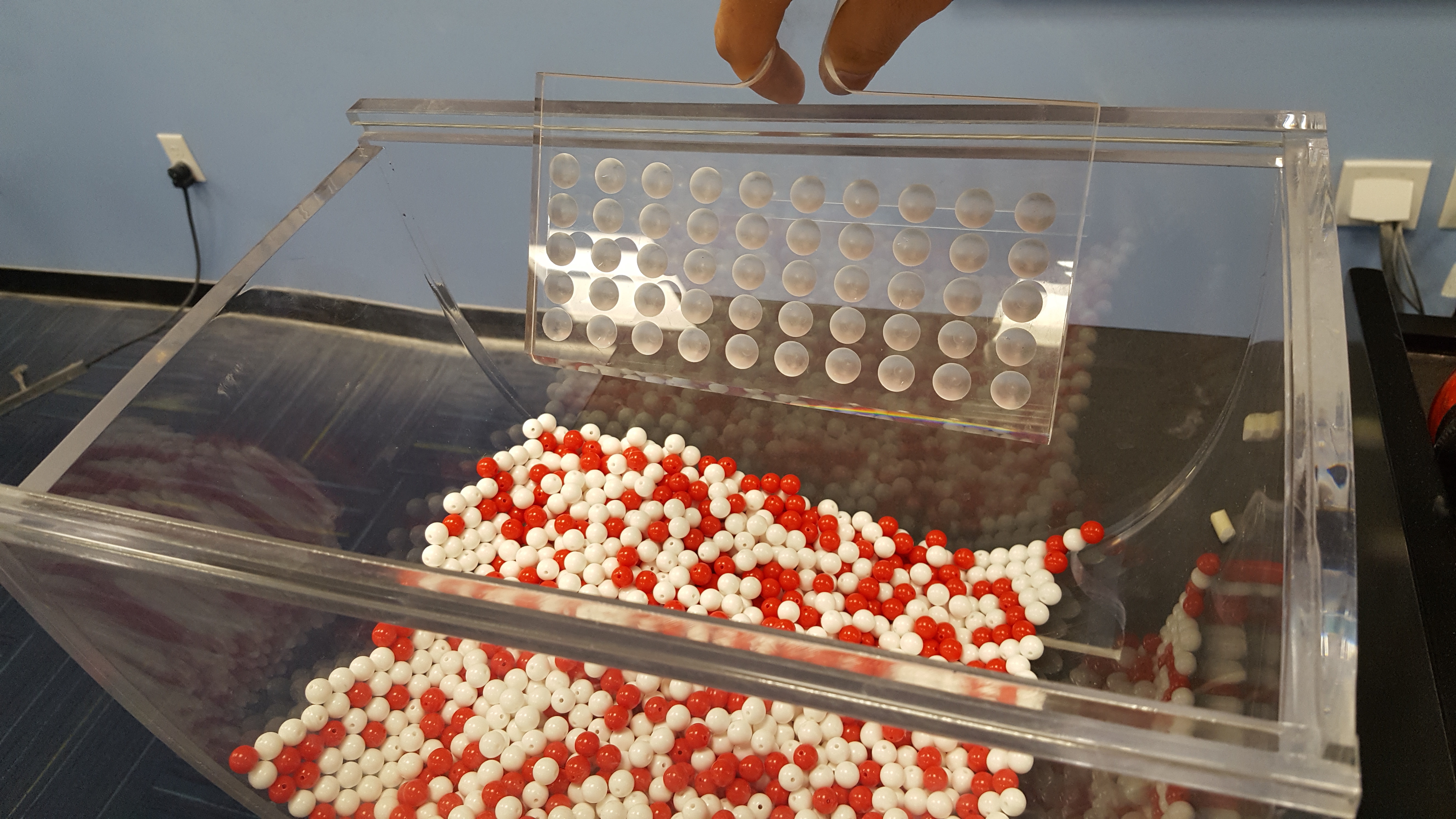
Figure 8.1: A bowl with 2400 balls

… and extract a sample of 50 balls:

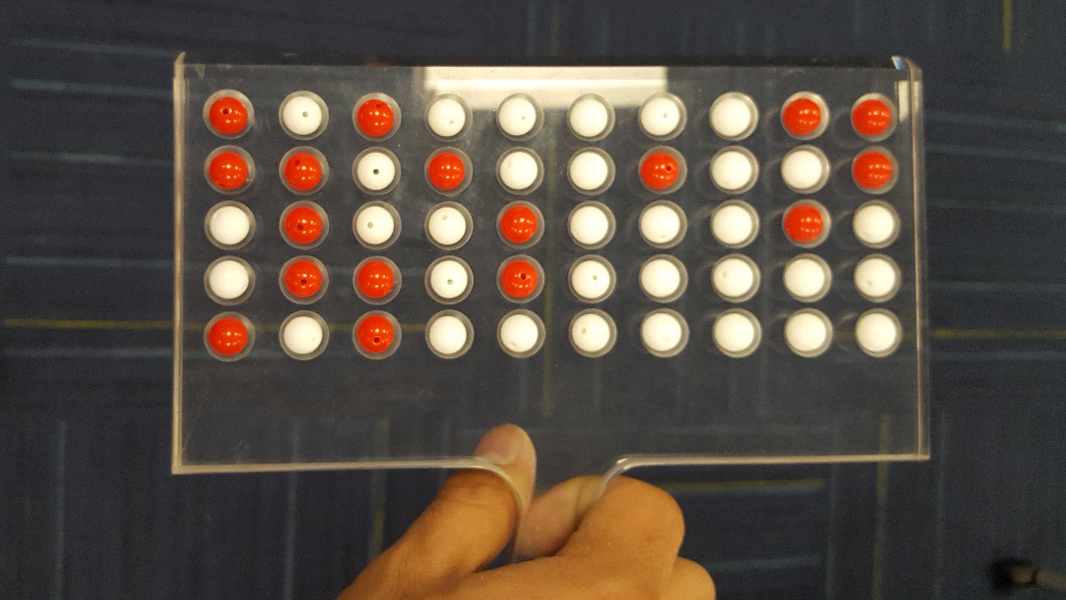
Figure 8.2: A shovel used to extract a sample of size n = 50

Concepts related to sampling

Let’s now define some concepts and terminology important to understand sampling, being sure to tie things back to the above example. You might have to read this a couple times more as you progress throughout this book, as they are very deeply layered concepts. However as we’ll soon see, they are very powerful concepts that open up a whole new world of scientific thinking:

Population: The population is a set of $N$ observations of interest.
- Above Ex: Our bowl consisting of $N=2400$ identically-shaped balls.
Population parameter: A population parameter is a numerical summary value about the population. In most settings, this is a value that’s unknown and you wish you knew it.
- Above Ex: The true population proportion $p$ of the balls in the bowl that are red.
- In this scenario the parameter of interest is the proportion, but in others it could be numerical summary values like the mean, median, etc.
Census: An exhaustive enumeration/counting of all observations in the population in order to compute the population parameter’s numerical value. exactly
- Above Ex: This corresponds to manually going over all $N=2400$ balls and counting the number that are red, thereby allowing us to compute the population proportion $p$ of the balls that are red exactly.
- When $N$ is small, a census is feasible. However, when $N$ is large, a census can get very expensive, either in terms of time, energy, or money.
- Ex: the Decennial United States census attempts to exhaustively count the US population. Consequently it is a very expensive, but necessary, procedure.
Sampling: Collecting a sample of size $n$ of observations from the population. Typically the sample size $n$ is much smaller than the population size $N$, thereby making sampling a much cheaper procedure than a census.
- Above Ex: Using the shovel to extract a sample of $n=50$ balls.
- It is important to remember that the lowercase $n$ corresponds to the sample size and uppercase $N$ corresponds to the population size, thus $n \leq N$.
Point estimates/sample statistics: A summary statistic based on the sample of size $n$ that estimates the unknown population parameter.
- Above Ex: it’s the sample proportion $\widehat{p}$ red of the balls in the sample of size $n=50$.
- Key: The sample proportion red $\widehat{p}$ is an estimate of the true unknown population proportion red $p$.
Representative sampling: A sample is said be a representative sample if it “looks like the population”. In other words, the sample’s characteristics are a good representation of the population’s characteristics.
- Above Ex: Does our sample of $n=50$ balls “look like” the contents of the larger set of $N=2400$ balls in the bowl?
Generalizability: We say a sample is generalizable if any results of based on the sample can generalize to the population.
- Above Ex: Is $\widehat{p}$ a “good guess” of $p$?
- In other words, can we infer about the true proportion of the balls in the bowl that are red, based on the results of our sample of $n=50$ balls?
Bias: In a statistical sense, we say bias occurs if certain observations in a population have a higher chance of being sampled than others. We say a sampling procedure is unbiased if every observation in a population had an equal chance of being sampled.
- Above Ex: Did each ball, irrespective of color, have an equal chance of being sampled, meaning the sampling was unbiased? we feel since the balls are all of the same size, there isn’t any bias in the sampling. If, say, the red balls had a much larger diameter than the red ones. You might have have a higher or lower probability of now sampling red balls.
Random sampling: We say a sampling procedure is random if we sample randomly from the population in an unbiased fashion.
- Above Ex: As long as you mixed the bowl sufficiently before sampling, your samples of size $n=50$ balls would be random.

Inference via sampling

Why did we go through the trouble of enumerating all the above concepts and terminology?

The moral of the story:

If the sampling of a sample of size $n$ is done at random, then

The sample is unbiased and representative of the population, thus

Any result based on the sample can generalize to the population, thus

The point estimate/sample statistic is a “good guess” of the unknown population parameter of interest

and thus we have inferred about the population based on our sample. In the above example:

If we properly mix the balls by say stirring the bowl first, then use the shovel to extract a sample of size $n=50$, then

The contents of the shovel will “look like” the contents of the bowl, thus

Any results based on the sample of $n=50$ balls can generalize to the large bowl of $N=2400$ balls, thus

The sample proportion $\widehat{p}$ of the $n=50$ balls in the shovel that are red is a “good guess” of the true population proportion $p$ of the $N=2400$ balls that are red.

and thus we have inferred some new piece of information about the bowl based on our sample extracted by shovel.

At this point, you might be saying to yourself: “Big deal, why do we care about this bowl?” As hopefully you’ll soon come to appreciate, this sampling bowl exercise is merely a simulation representing the reality of many important sampling scenarios in a simplified and accessible setting. One in particular sampling scenario is familiar to many: polling. Whether for market research or for political purposes, polls inform much of the world’s decision and opinion making, and understanding the mechanism behind them can better inform you statistical citizenship. We’ll tie-in everything we learn in this chapter with an example relating to a 2013 poll on President Obama’s approval ratings among young adult in Section 8.4.

8.2 Tactile sampling simulation

Let’s start by revisiting our tactile sampling illustrating with “sampling bowl” in Figures 8.1 and 8.2. By tactile we mean with your hands and to the touch. We’ll break down the act of tactile sampling from the bowl with the shovel using our newly acquired concepts and terminology relating to sampling. In particular we’ll study how sampling variability affects outcomes, which we’ll illustrate through simulations of repeated sampling. To this end, we’ll be using both the above-mentioned tactile simulation, but also using virtual simulation. By virtual we mean on the computer.

8.2.1 Using shovel once

Let’s now view our shovel through the lens of sampling with the following 3-step tactile sampling simulation:

Step 1: Use the shovel to take a sample of size $n=50$ balls from the bowl as seen in Fig 8.3.

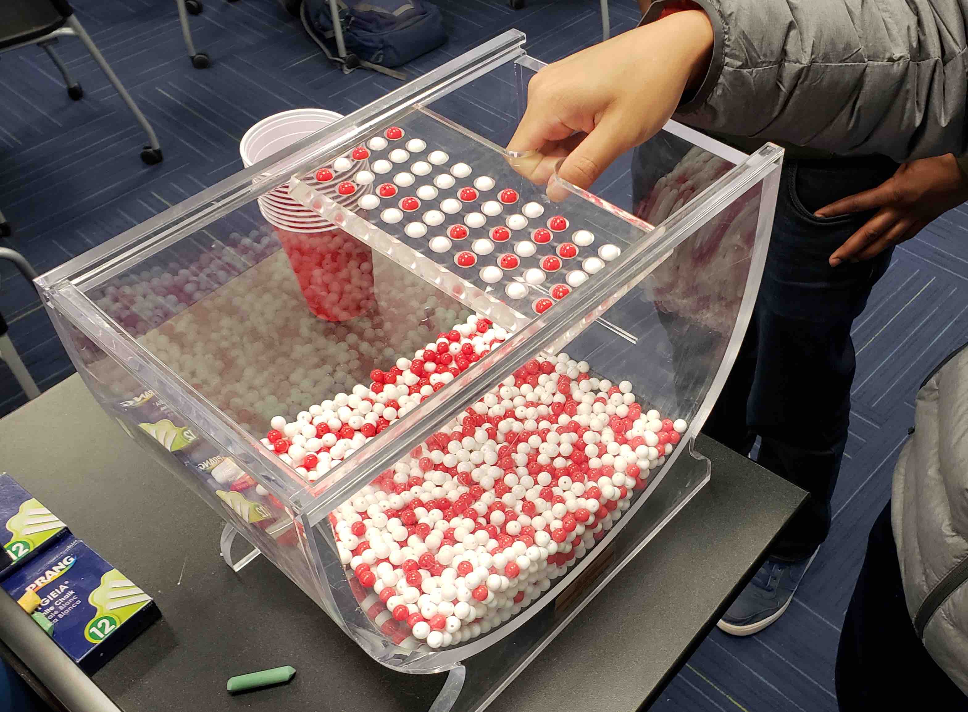
Figure 8.3: Step 1: Take sample of size $n=50$

Step 2: Pour them into a cup and

Count the number that are red then
Compute the sample proportion $\widehat{p}$ of the $n=50$ balls that are red

as seen in Figure 8.4 below. Note from above there are 18 balls out of $n=50$ that are red. Thus the sample proportion red $\widehat{p}$ for this particular sample is thus $\widehat{p} = 18 / 50 = 0.36$.

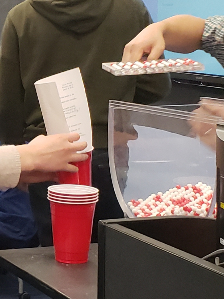
$Step 2: Pour into Red Solo Cup and compute $\widehat{p}$$

Figure 8.4: Step 2: Pour into Red Solo Cup and compute $\widehat{p}$

Step 3: Mark the sample proportion $\widehat{p}$ in a hand-drawn histogram, just like our intrepid students are doing in Figure 8.5.

$Step 3: Mark $\widehat{p}$'s in histogram$

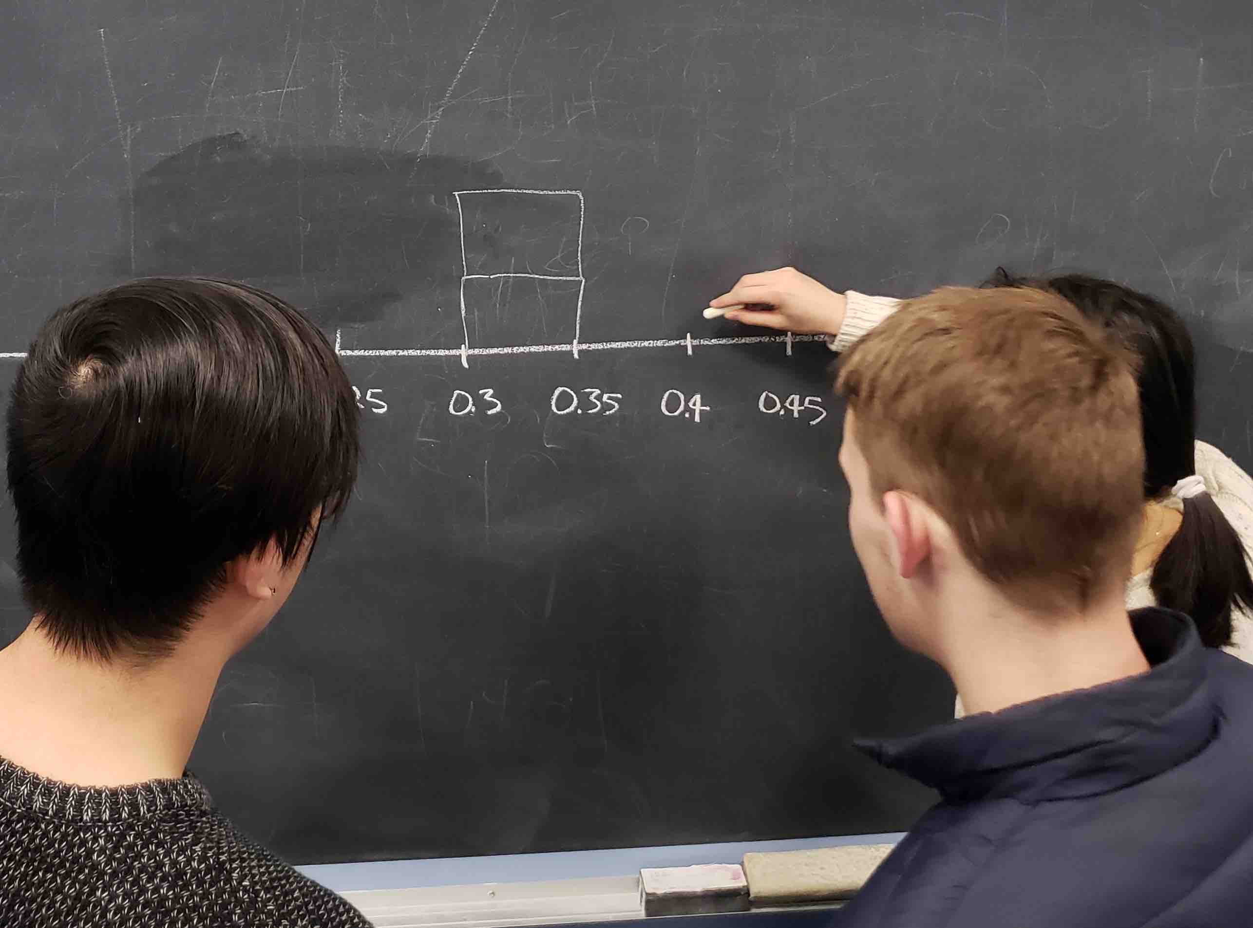
Figure 8.5: Step 3: Mark $\widehat{p}$’s in histogram

Repeat Steps 1-3 a few times: After a few groups of students complete this exercise, let’s draw the resulting histogram by hand. In Figure 8.6 we have the resulting hand-drawn histogram for 10 groups of students.

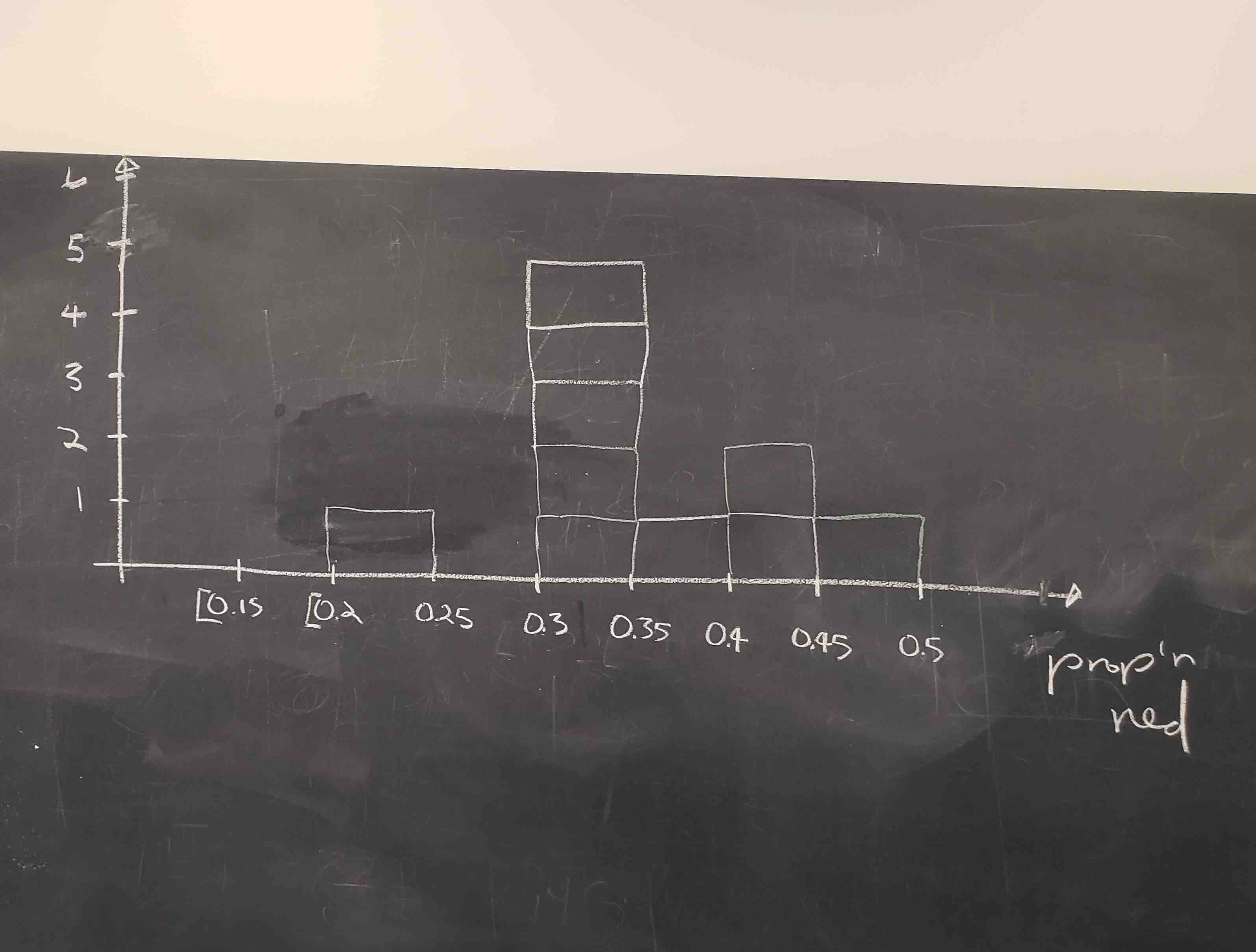
$Step 3: Histogram of 10 values of $\widehat{p}$$

Figure 8.6: Step 3: Histogram of 10 values of $\widehat{p}$

Observe the behavior of the 10 different values of the sample proportion $\widehat{p}$ in the histogram of their distribution, in particular where the values center and how much they spread out, in other words how much they vary. Note:

The lowest value of $\widehat{p}$ was somewhere between 0.20 and 0.25.
The highest value of $\widehat{p}$ was somewhere between 0.45 and 0.50.
Five of the sample proportions $\widehat{p}$ cluster. Five different samples of size $n=50$ yielded sample proportions $\widehat{p}$ that were in the range 0.30 to 0.35.

Let’s now look at some real-life outcomes of this tactile sampling simulation. We present the actual results for not 10 groups of students, but 33 groups of students below!

8.2.2 Using shovel 33 times

All told, 33 groups took samples. In other words, the shovel was used 33 times and 33 values of the sample proportion $\widehat{p}$ were computed; this data is saved in the tactile_prop_red data frame included in the moderndive package. Let’s display its contents in Table ??. Notice how the replicate column enumerates each of the 33 groups, red_balls is the count of balls in the sample of size $n=50$ that we red, and prop_red is the sample proportion $\widehat{p}$ that are red.

tactile_prop_red
View(tactile_prop_red)

group	replicate	red_balls	prop_red
Ilyas, Yohan	1	21	0.42
Morgan, Terrance	2	17	0.34
Martin, Thomas	3	21	0.42
Clark, Frank	4	21	0.42
Riddhi, Karina	5	18	0.36
Andrew, Tyler	6	19	0.38
Julia	7	19	0.38
Rachel, Lauren	8	11	0.22
Daniel, Caroline	9	15	0.30
Josh, Maeve	10	17	0.34
Emily, Emily	11	16	0.32
Conrad, Emily	12	18	0.36
Oliver, Erik	13	17	0.34
Isabel, Nam	14	21	0.42
X, Claire	15	15	0.30
Cindy, Kimberly	16	20	0.40
Kevin, James	17	11	0.22
Nam, Isabelle	18	21	0.42
Harry, Yuko	19	15	0.30
Yuki, Eileen	20	16	0.32
Ramses	21	23	0.46
Joshua, Elizabeth, Stanley	22	15	0.30
Siobhan, Jane	23	18	0.36
Jack, Will	24	16	0.32
Caroline, Katie	25	21	0.42
Griffin, Y	26	18	0.36
Kaitlin, Jordan	27	17	0.34
Ella, Garrett	28	18	0.36
Julie, Hailin	29	15	0.30
Katie, Caroline	30	21	0.42
Mallory, Damani, Melissa	31	21	0.42
Katie	32	16	0.32
Francis, Vignesh	33	19	0.38

Using your data visualization skills that you honed in Chapter 3, let’s visualize the distribution of these 33 sample proportions red $\widehat{p}$ using a histogram with binwidth = 0.05. This visualization is appropriate since prop_red is a numerical variable. This histogram is showing a very particular important type of distribution in statistics: the sampling distribution.

ggplot(tactile_prop_red, aes(x = prop_red)) +
  geom_histogram(binwidth = 0.05, color = "white") +
  labs(x = "Sample proportion red based on n = 50", title = "Sampling distribution of p-hat")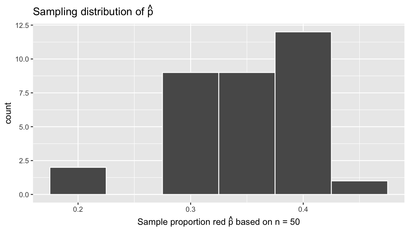

Figure 8.7: Sampling distribution of 33 sample proportions based on 33 tactile samples with n=50

Sampling distributions are a specific kind of distribution: distributions of point estimates/sample statistics based on samples of size $n$ used to estimate an unknown population parameter.

In the case of the histogram in Figure 8.7, its the distribution of the sample proportion red $\widehat{p}$ based on $n=50$ sampled balls from the bowl, for which we want to estimate the unknown population proportion $p$ of the $N=2400$ balls that are red. Sampling distributions describe how values of the sample proportion red $\widehat{p}$ will vary from sample to sample due to sampling variability and thus identify “typical” and “atypical” values of $\widehat{p}$. For example

Obtaining a sample that yields $\widehat{p} = 0.36$ would be considered typical, common, and plausible since it would in theory occur frequently.
Obtaining a sample that yields $\widehat{p} = 0.8$ would be considered atypical, uncommon, and implausible since it lies far away from most of the distribution.

Let’s now ask ourselves the following questions:

Where is the sampling distribution centered?
What is the spread of this sampling distribution?

Recall from Section 5.4 the mean and the standard deviation are two summary statistics that would answer this question:

tactile_prop_red %>% 
  summarize(mean = mean(prop_red), sd = sd(prop_red))

mean	sd
0.356	0.058

Finally, it’s important to keep in mind:

If the sampling is done in an unbiased and random fashion, in other words we made sure to stir the bowl before we sampled, then the sampling distribution will be guaranteed to be centered at the true unknown population proportion red $p$, or in other words the true number of balls out of 2400 that are red.
The spread of this histogram, as quantified by the standard deviation of 0.058, is called the standard error. It quantifies the variability of our estimates for $\widehat{p}$.
- Note: A large source of confusion. All standard errors are a form of standard deviation, but not all standard deviations are standard errors.

8.3 Virtual sampling simulation

Now let’s mimic the above tactile sampling, but with virtual sampling. We’ll resort to virtual sampling because while collecting 33 tactile samples manually is feasible, for large numbers like 1000, things start getting tiresome! That’s where a computer can really help: computers excel at performing mundane tasks repeatedly; think of what accounting software must be like!

In other words:

Instead of considering the tactile bowl shown in Figure 8.1 above and using a tactile shovel to draw samples of size $n=50$
Let’s use a virtual bowl saved in a computer and use R’s random number generator as a virtual shovel to draw samples of size $n=50$

First, we describe our virtual bowl. In the moderndive package, we’ve included a data frame called bowl that has 2400 rows corresponding to the $N=2400$ balls in the physical bowl. Run View(bowl) in RStudio to convince yourselves that bowl is indeed a virtual version of the tactile bowl in the previous section.

bowl

# A tibble: 2,400 x 2
   ball_ID color
     <int> <chr>
 1       1 white
 2       2 white
 3       3 white
 4       4 red  
 5       5 white
 6       6 white
 7       7 red  
 8       8 white
 9       9 red  
10      10 white
# … with 2,390 more rows

Note that the balls are not actually marked with numbers; the variable ball_ID is merely used as an identification variable for each row of bowl. Recall our previous discussion on identification variables in Subsection 4.2.2 in the “Data Tidying” Chapter 4.

Next, we describe our virtual shovel: the rep_sample_n() function included in the moderndive package where rep_sample_n() indicates that we are taking repeated/replicated samples of size $n$.

8.3.1 Using shovel once

The rep_sample_n() function included in the moderndive package where rep_sample_n() indicates that we are taking repeated/replicated samples of size $n$. Let’s perform the virtual analogue of tactilely inserting the shovel only once into the bowl and extracting a sample of size $n=50$. In the table below we only show results about the first 10 sampled balls out of 50.

virtual_shovel <- bowl %>% 
  rep_sample_n(size = 50)
View(virtual_shovel)

Table 8.1: First 10 sampled balls of 50 in virtual sample
replicate	ball_ID	color
1	2079	red
1	1076	white
1	1691	red
1	1687	red
1	1434	white
1	954	white
1	483	white
1	1520	white
1	2060	red
1	1682	white

Looking at all 50 rows of virtual_shovel in the spreadsheet viewer that pops up after running View(virtual_shovel) in RStudio, the ball_ID variable seems to suggest that we do indeed have a random sample of $n=50$ balls. However, what does the replicate variable indicate, where in this case it’s equal to 1 for all 50 rows? We’ll see in a minute. First let’s compute both the number of balls red and the proportion red out of $n=50$ using our dplyr data wrangling tools from Chapter 5:

virtual_shovel %>% 
  summarize(red = sum(color == "red")) %>% 
  mutate(prop_red = red / 50)

Table 8.2: Count and proportion red in single virtual sample of size n = 50
replicate	red	prop_red
1	23	0.46

Why does this work? Because for every row where color == "red", the Boolean TRUE is returned and R treats TRUE like the number 1. Equivalently, for every row where color is not equal to "red", the Boolean FALSE is returned and R treats FALSE like the number 0. So summing the number of TRUE’s and FALSE’s is equivalent to summing 1’s and 0’s which counts the number of balls where color is red.

8.3.2 Using shovel 33 times

Recall however in our tactile sampling exercise in Section 8.2 above that we had 33 groups of students take 33 samples total of size $n=50$ using the shovel 33 times and hence compute 33 separate values of the sample proportion red $\widehat{p}$. In other words we repeated/replicated the sampling 33 times. We can achieve this by reusing the same rep_sample_n() function code above, but by adding the reps = 33 argument indicating we want to repeat this sampling 33 times:

virtual_samples <- bowl %>% 
  rep_sample_n(size = 50, reps = 33)
View(virtual_samples)

virtual_samples has $50 \times 33 = 1650$ rows, corresponding to 33 samples of size $n=50$, or 33 draws from the shovel. We won’t display the contents of this data frame but leave it to you to View() this data frame. You’ll see that the first 50 rows have replicate equal to 1, then the next 50 rows have replicate equal to 2, and so on and so forth, up until the last 50 rows which have replicate equal to 33. The replicate variable denotes which of our 33 samples a particular ball is included in.

Now let’s compute the 33 corresponding values of the sample proportion $\widehat{p}$ based on 33 different samples of size $n=50$ by reusing the previous code, but remembering to group_by the replicate variable first since we want to compute the sample proportion for each of the 33 samples separately. Notice the similarity of this table with Table ??.

virtual_prop_red <- virtual_samples %>% 
  group_by(replicate) %>% 
  summarize(red = sum(color == "red")) %>% 
  mutate(prop_red = red / 50)
View(virtual_prop_red)

replicate	red	prop_red
1	17	0.34
2	20	0.40
3	24	0.48
4	20	0.40
5	17	0.34
6	16	0.32
7	17	0.34
8	19	0.38
9	19	0.38
10	12	0.24
11	22	0.44
12	17	0.34
13	20	0.40
14	22	0.44
15	13	0.26
16	15	0.30
17	23	0.46
18	20	0.40
19	16	0.32
20	12	0.24
21	14	0.28
22	21	0.42
23	14	0.28
24	18	0.36
25	19	0.38
26	12	0.24
27	22	0.44
28	23	0.46
29	19	0.38
30	18	0.36
31	20	0.40
32	17	0.34
33	20	0.40

Just as we did before, let’s now visualize the sampling distribution using a histogram with binwidth = 0.05 of the 33 virtually sample proportions $\widehat{p}$:

ggplot(virtual_prop_red, aes(x = prop_red)) +
  geom_histogram(binwidth = 0.05, color = "white") +
  labs(x = "Sample proportion red based on n = 50", title = "Sampling distribution of p-hat")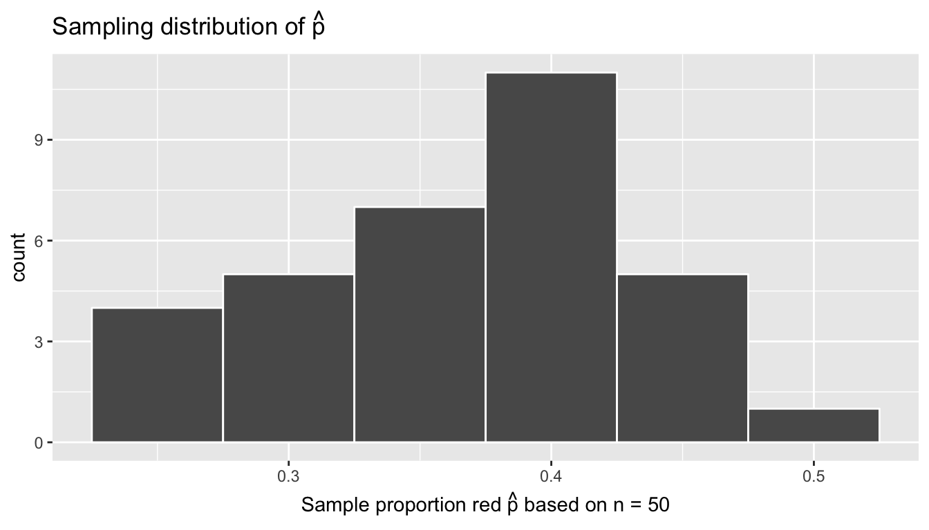

Figure 8.8: Sampling distribution of 33 sample proportions based on 33 virtual samples with n=50

The resulting sampling distribution based on our virtual sampling simulation is near identical to the sampling distribution of our tactile sampling simulation from Section 8.3. Let’s compare them side-by-side in Figure 8.9.

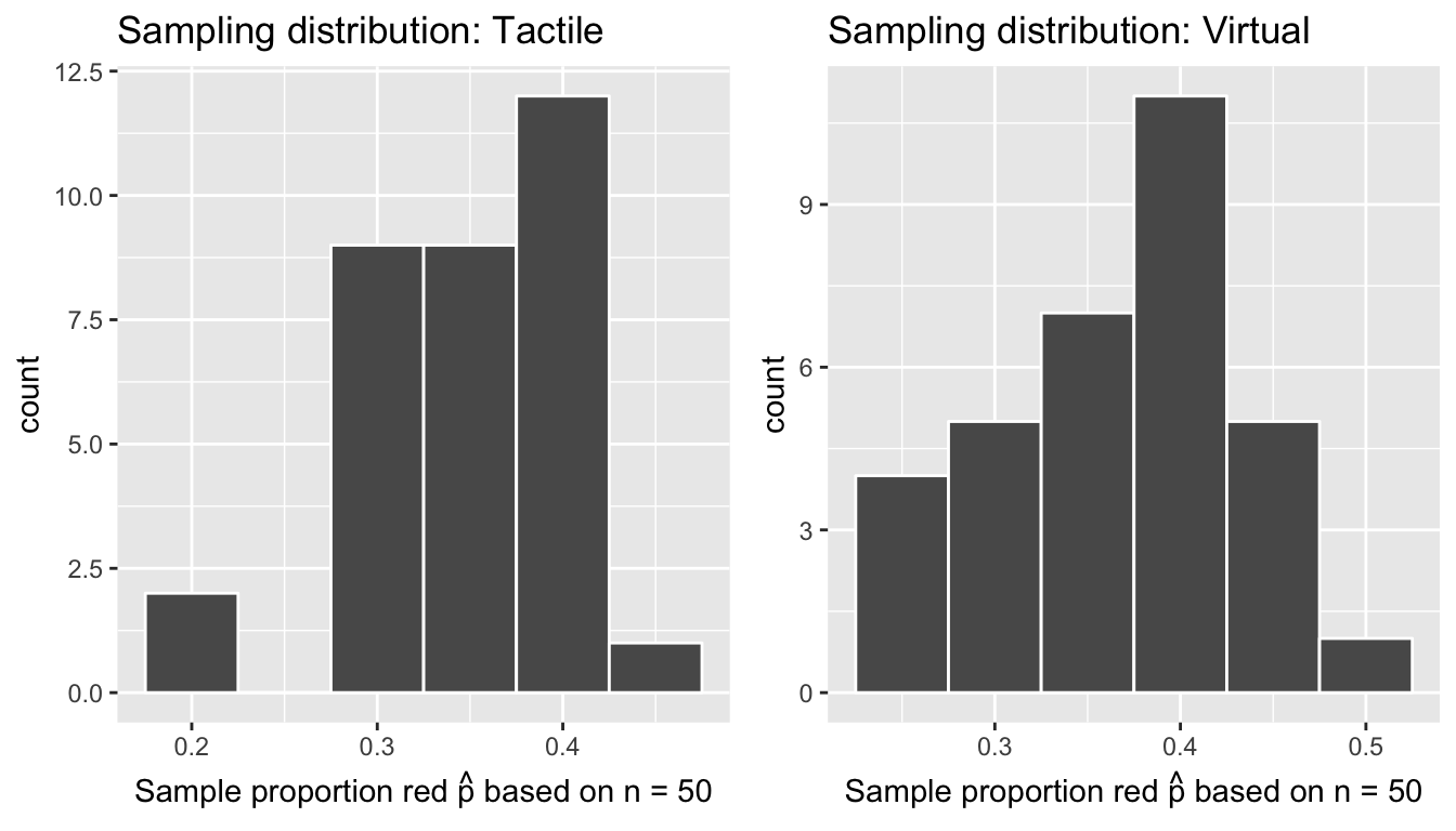
Figure 8.9: Comparison of sampling distributions based on 33 tactile & virtual samples with n=50

We see that they are similar in terms of center and spread, although not identical due to random variation. This was in fact by design, as we made the virtual contents of the virtual bowl match the actual contents of the actual bowl pictured above.

8.3.3 Using shovel 1000 times

In Figure 8.8, we can start seeing a pattern in the sampling distribution emerge. However, 33 values of the sample proportion $\widehat{p}$ might not be enough to get a true sense of the distribution. Using 1000 values of $\widehat{p}$ would definitely give a better sense. What are our two options for constructing these histograms?

Tactile sampling: Make the 33 groups of students take $1000 / 33 \approx 31$ samples of size $n=50$ each, count the number of red balls for each of the 1000 tactile samples, and then compute the 1000 corresponding values of the sample proportion $\widehat{p}$. However, this would be cruel and unusual as this would take hours!
Virtual sampling: Computers are very good at automating repetitive tasks such as this one. This is the way to go!

First, generate 1000 samples of size $n=50$

virtual_samples <- bowl %>% 
  rep_sample_n(size = 50, reps = 1000)
View(virtual_samples)

Then for each of these 1000 samples of size $n=50$, compute the corresponding sample proportions

virtual_prop_red <- virtual_samples %>% 
  group_by(replicate) %>% 
  summarize(red = sum(color == "red")) %>% 
  mutate(prop_red = red / 50)
View(virtual_prop_red)

As previously done, let’s plot the sampling distribution of these 1000 simulated values of the sample proportion red $\widehat{p}$ with a histogram in Figure 8.10.

ggplot(virtual_prop_red, aes(x = prop_red)) +
  geom_histogram(binwidth = 0.05, color = "white") +
  labs(x = "Sample proportion red based on n = 50", title = "Sampling distribution of p-hat")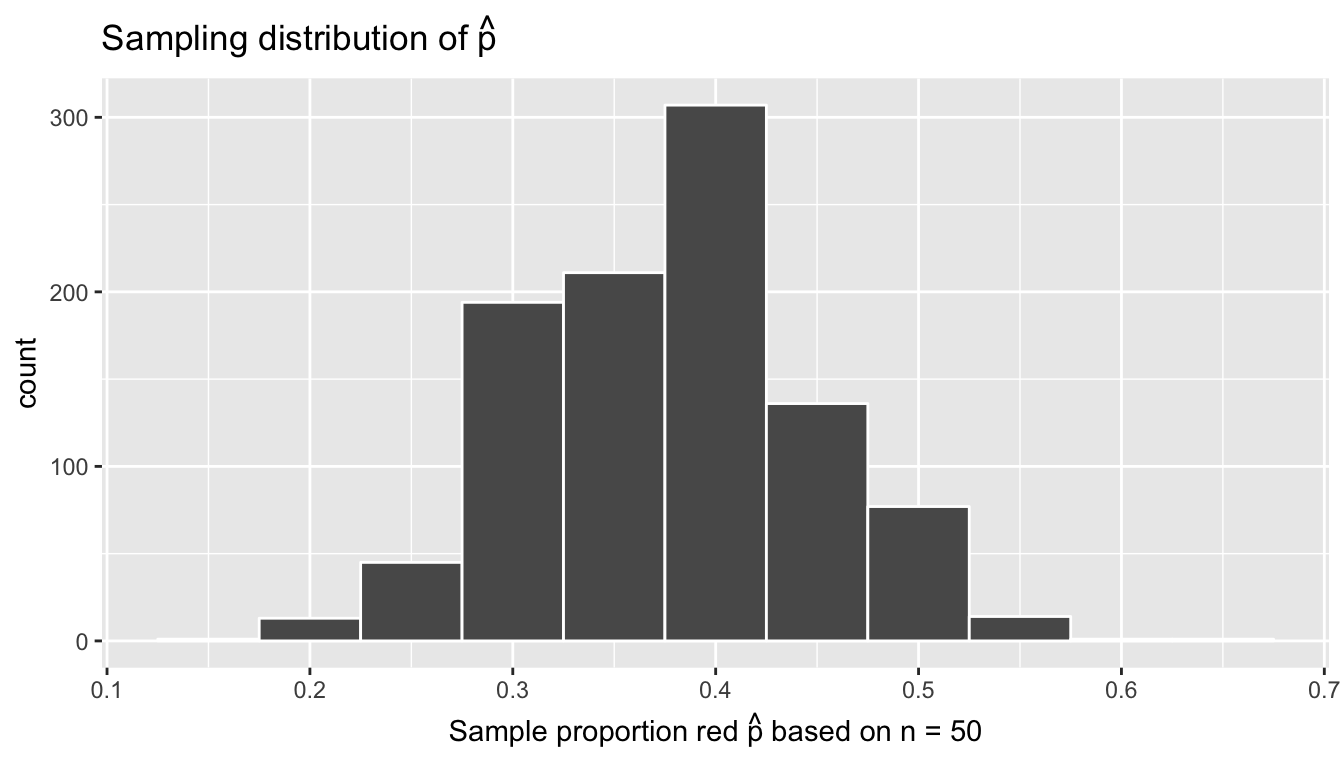

Figure 8.10: Sampling distribution of 1000 sample proportions based on 1000 tactile samples with n=50

Since the sampling is random and thus representative and unbiased, the above sampling distribution is centered at the true population proportion red $p$ of all $N=2400$ balls in the bowl. Eyeballing it, the sampling distribution appears to be centered at around 0.375.

What is the standard error of the above sampling distribution of $\widehat{p}$ based on 1000 samples of size $n=50$?

virtual_prop_red %>% 
  summarize(SE = sd(prop_red))

# A tibble: 1 x 1
      SE
   <dbl>
1 0.0698

What this value is saying might not be immediately apparent by itself to someone who is new to sampling. It’s best to first compare different standard errors for different sampling schemes based on different sample sizes $n$. We’ll do so for samples of size $n=25$, $n=50$, and $n=100$ next.

8.3.4 Using different shovels

Recall, the sampling we just did on the computer using the rep_sample_n() function is simply a virtual version of act of taking a tactile sample using the shovel with $n=50$ slots seen in Figure 8.11. We visualized the variation in the resulting sample proportion red $\widehat{p}$ in a histogram of the sampling distribution and quantified this variation using the standard error.

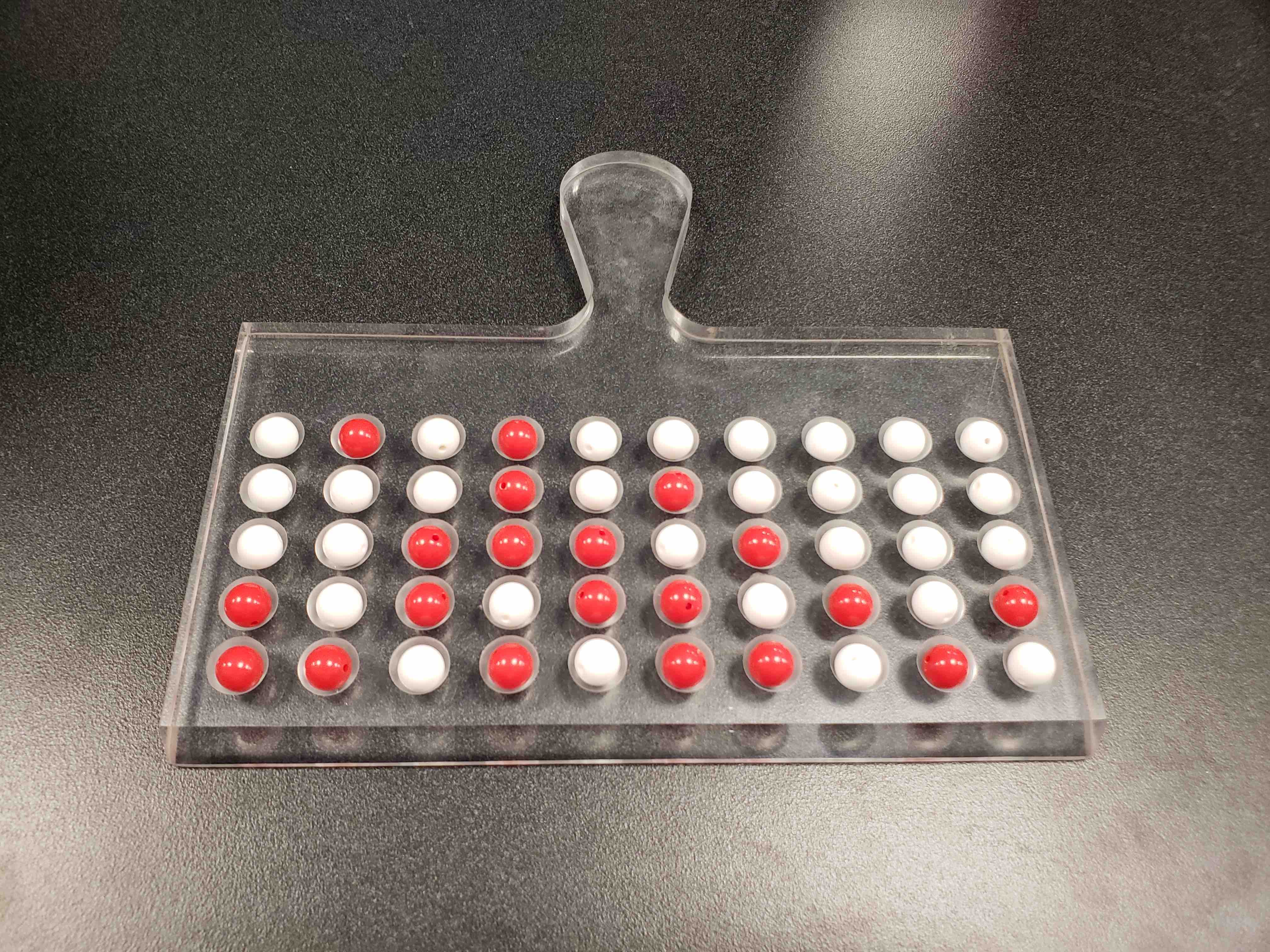
Figure 8.11: Tactile shovel for sampling n = 50 balls

But what if we changed the sample size to $n=25$? This would correspond to sampling using the shovel with $n=25$ slots see in Figure 8.12. What differences if any would you notice about the sampling distribution and the standard error?

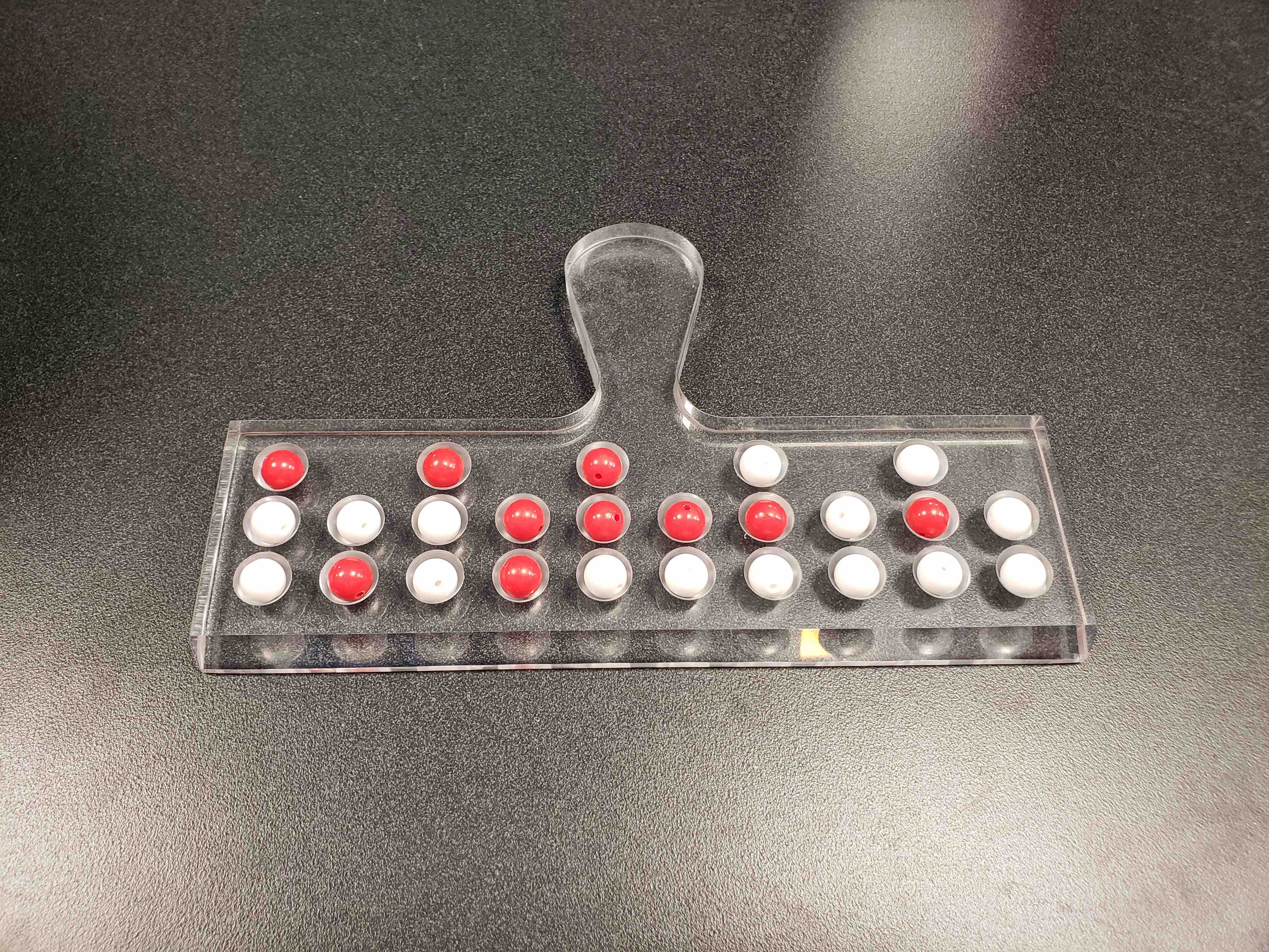
Figure 8.12: Tactile shovel for sampling n = 25 balls

Furthermore what if we took samples of size $n=100$ as well? This would correspond to sampling using the shovel with $n=100$ slots see in Figure 8.13. What differences if any would you notice about the sampling distribution and the standard error for $n=100$ as compared to $n=50$ and $n=25$?

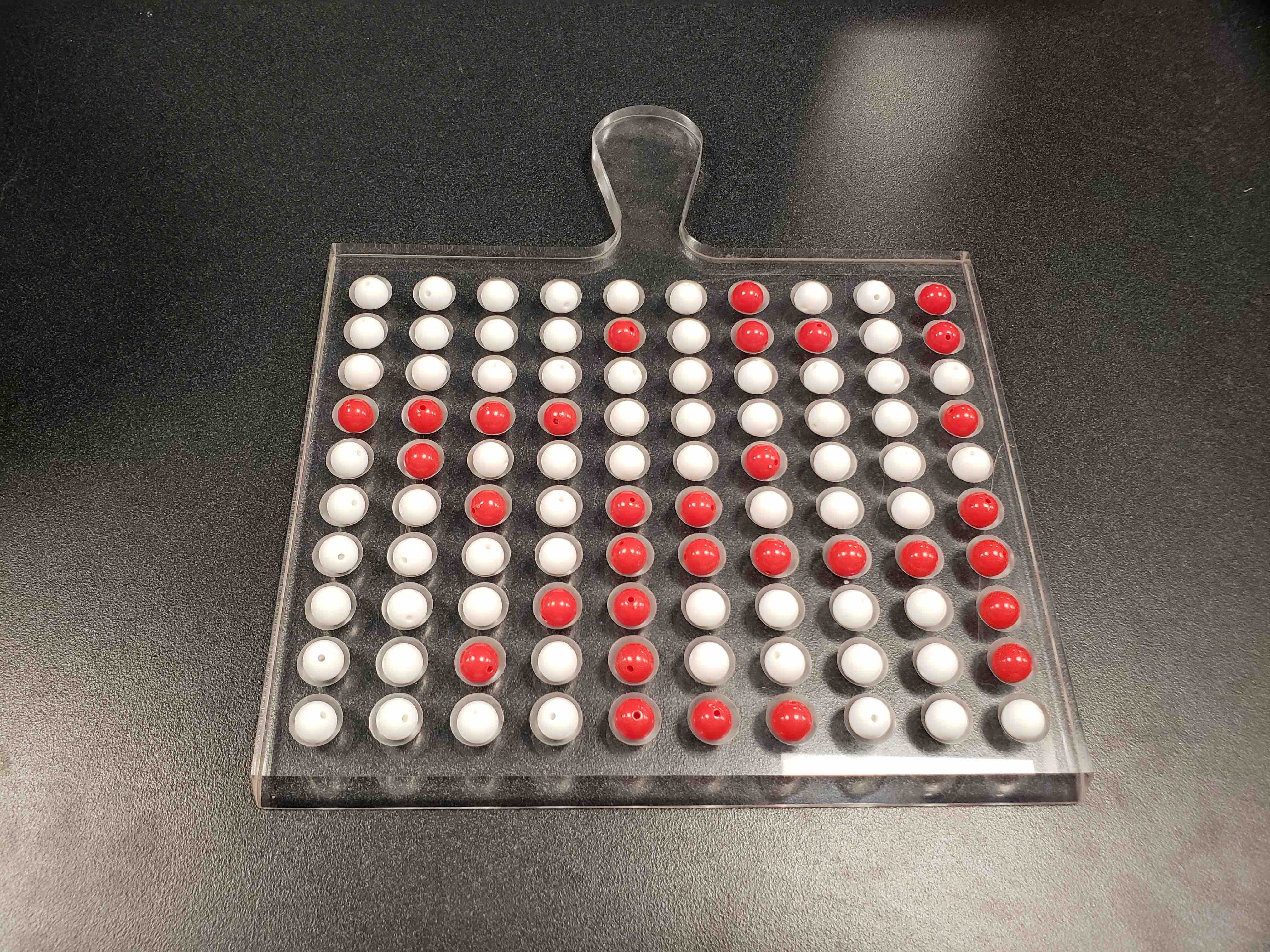
Figure 8.13: Tactile shovel for sampling n = 100 balls

Let’s take the opportunity to review our sampling procedure and do this for 1000 virtual samples of size $n=25$, $n=50$, $n=100$ each.

Shovel with $n=50$ slots: Take 1000 virtual samples of size $n=50$, mimicking the act of taking 1000 tactile samples using the shovel with $n=50$ slots:

virtual_samples_50 <- bowl %>% 
  rep_sample_n(size = 50, reps = 1000)

Then based on each of these 1000 virtual samples of size $n=50$, compute the corresponding 1000 sample proportions $\widehat{p}$ being sure to divide by 50:

virtual_prop_red_50 <- virtual_samples_50 %>% 
  group_by(replicate) %>% 
  summarize(red = sum(color == "red")) %>% 
  mutate(prop_red = red / 50)

The standard error is the standard deviation of the 1000 sample proportions $\widehat{p}$, in other words we are quantifying how much $\widehat{p}$ varies from sample-to-sample based on samples of size $n=50$ due to sampling variation.

virtual_prop_red_50 %>% 
  summarize(SE = sd(prop_red))

# A tibble: 1 x 1
      SE
   <dbl>
1 0.0694

Shovel with $n=25$ slots: Take 1000 virtual samples of size $n=25$, mimicking the act of taking 1000 tactile samples using the shovel with $n=25$ slots:

virtual_samples_25 <- bowl %>% 
  rep_sample_n(size = 25, reps = 1000)

Then based on each of these 1000 virtual samples of size $n=50$, compute the corresponding 1000 sample proportions $\widehat{p}$ being sure to divide by 50:

virtual_prop_red_25 <- virtual_samples_25 %>% 
  group_by(replicate) %>% 
  summarize(red = sum(color == "red")) %>% 
  mutate(prop_red = red / 25)

virtual_prop_red_25 %>% 
  summarize(SE = sd(prop_red))

# A tibble: 1 x 1
     SE
  <dbl>
1 0.100

Shovel with $n=100$ slots: Take 1000 virtual samples of size $n=100$, mimicking the act of taking 1000 tactile samples using the shovel with $n=100$ slots:

virtual_samples_100 <- bowl %>% 
  rep_sample_n(size = 100, reps = 1000)

Then based on each of these 1000 virtual samples of size $n=100$, compute the corresponding 1000 sample proportions $\widehat{p}$ being sure to divide by 100:

virtual_prop_red_100 <- virtual_samples_100 %>% 
  group_by(replicate) %>% 
  summarize(red = sum(color == "red")) %>% 
  mutate(prop_red = red / 100)

virtual_prop_red_100 %>% 
  summarize(SE = sd(prop_red))

# A tibble: 1 x 1
      SE
   <dbl>
1 0.0457

Comparison: Let’s compare the 3 standard errors we computed above in Table ??:

n	SE
25	0.100
50	0.069
100	0.046

Observe the behavior of the standard error as $n$ increases from $n=25$ to $n=50$ to $n=100$, the standard error get smaller. In other words, the values of $\widehat{p}$ vary less. The standard error is a numerical quantification of the spreads of the following three histograms (on the same scale) of the sampling distribution of the sample proportion $\widehat{p}$:

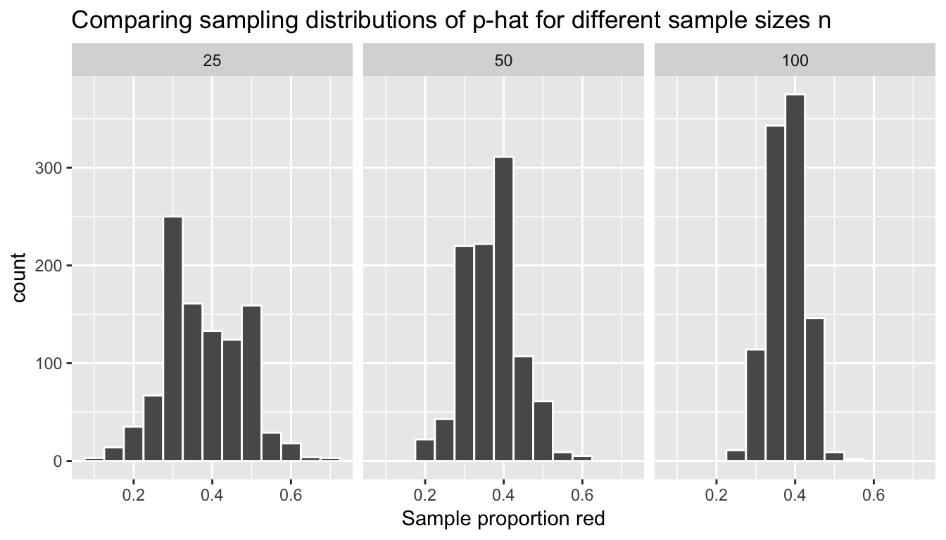
Figure 8.14: Comparing sampling distributions of p-hat for different sample sizes n

Observe that the histogram of possible $\widehat{p}$ values are narrowest and most consistent for the $n=100$ case. In other words, they make less error. “Bigger sample size equals better sampling” is a concept you probably knew before reading this chapter. What we’ve just demonstrated is what this concept means: Samples based on large samples sizes will yield point estimates that vary less around the true value and hence be less prone to error.

In the case of our sampling bowl, the sample proportion red $\widehat{p}$ based on samples of size $n=100$ will vary the least around the true proportion $p$ of the balls that are red, and thus be less prone to error. On the case of polls as we study in the next chapter: representative polls based on a larger number of respondents will yield guess that tend to be closer to the truth.

8.4 In real-life sampling: Polls

In December 4, 2013 National Public Radio reported on a recent poll of President Obama’s approval rating among young Americans aged 18-29 in an article Poll: Support For Obama Among Young Americans Eroding. A quote from the article:

After voting for him in large numbers in 2008 and 2012, young Americans are souring on President Obama.

According to a new Harvard University Institute of Politics poll, just 41 percent of millennials — adults ages 18-29 — approve of Obama’s job performance, his lowest-ever standing among the group and an 11-point drop from April.

Let’s tie elements of this story using the concepts and terminology we learned at the outset of this chapter along with our observations from the tactile and virtual sampling simulations:

Population: Who is the population of $N$ observations of interest?
- Bowl: $N=2400$ identically-shaped balls
- Obama poll: $N = \text{?}$ young Americans aged 18-29
Population parameter: What is the population parameter?
- Bowl: The true population proportion $p$ of the balls in the bowl that are red.
- Obama poll: The true population proportion $p$ of young Americans who approve of Obama’s job performance.
Census: What would a census be in this case?
- Bowl: Manually going over all $N=2400$ balls and exactly computing the population proportion $p$ of the balls that are red.
- Obama poll: Locating all $N = \text{?}$ young Americans (which is in the millions) and asking them if they approve of Obama’s job performance. This would be quite expensive to do!
Sampling: How do you acquire the sample of size $n$ observations?
- Bowl: Using the shovel to extract a sample of $n=50$ balls.
- Obama poll: One way would be to get phone records from a database and pick out $n$ phone numbers. In the case of the above poll, the sample was of size $n=2089$ young adults.
Point estimates/sample statistics: What is the summary statistic based on the sample of size $n$ that estimates the unknown population parameter?
- Bowl: The sample proportion $\widehat{p}$ red of the balls in the sample of size $n=50$.
- Key: The sample proportion red $\widehat{p}$ of young Americans in the sample of size $n=2089$ that approve of Obama’s job performance. In this study’s case, $\widehat{p} = 0.41$ which is the quoted 41% figure in the article.
Representative sampling: Is the sample procedure representative? In other words, to the resulting samples “look like” the population?
- Bowl: Does our sample of $n=50$ balls “look like” the contents of the larger set of $N=2400$ balls in the bowl?
- Obama poll: Does our sample of $n=2089$ young Americans “look like” the population of all young Americans aged 18-29?
Generalizability: Are the samples generalizable to the greater population?
- Bowl: Is $\widehat{p}$ a “good guess” of $p$?
- Obama poll: Is $\widehat{p} = 0.41$ a “good guess” of $p$? In other words, can we confidently say that 41% of all young Americans approve of Obama.
Bias: Is the sampling procedure unbiased? In other words, do all observations have an equal chance of being included in the sample?
- Bowl: Here, I would say it is unbiased. All balls are equally sized as evidenced by the slots of the $n=50$ shovel, and thus no particular color of ball can be favored in our samples over others.
- Obama poll: Did all young Americans have an equal chance at being represented in this poll? For example, if this was conducted using a database of only mobile phone numbers, would people without mobile phones be included? What about if this were an internet poll on a certain news website? Would non-readers of this this website be included?
Random sampling: Was the sampling random?
- Bowl: As long as you mixed the bowl sufficiently before sampling, your samples would be random?
- Obama poll: Random sampling is a necessary assumption for all of the above to work. Most articles reporting on polls take this assumption as granted. In our Obama poll, you’d have to ask the group that conducted the poll: The Harvard University Institute of Politics.

Recall the punchline of all the above:

If the sampling of a sample of size $n$ is done at random, then

The sample is unbiased and representative of the population, thus

Any result based on the sample can generalize to the population, thus

The point estimate/sample statistic is a “good guess” of the unknown population parameter of interest

and thus we have inferred about the population based on our sample. In the bowl example:

If we properly mix the balls by say stirring the bowl first, then use the shovel to extract a sample of size $n=50$, then

The contents of the shovel will “look like” the contents of the bowl, thus

Any results based on the sample of $n=50$ balls can generalize to the large bowl of $N=2400$ balls, thus

The sample proportion $\widehat{p}$ of the $n=50$ sampled balls in the shovel that are red is a “good guess” of the true population proportion $p$ of the $N=2400$ balls that are red.

and thus we have inferred some new piece of information about the bowl based on our sample extracted by shovel: the proportion of balls that are red. In the Obama poll example:

If we had a way of contacting a randomly chosen sample of 2089 young Americans and poll their approval of Obama, then

These 2089 young Americans would “look like” the population of all young Americans, thus

Any results based on this sample of 2089 young Americans can generalize to entire population of all young Americans, thus

The reported sample approval rating of 41% of these 2089 young Americans is a “good guess” of the true approval rating amongst all young Americans.

So long story short, this poll’s guess of Obama’s approval rating was 41%. However is this the end of the story when understanding the results of a poll? If you read further in the article, it states:

The online survey of 2,089 adults was conducted from Oct. 30 to Nov. 11, just weeks after the federal government shutdown ended and the problems surrounding the implementation of the Affordable Care Act began to take center stage. The poll’s margin of error was plus or minus 2.1 percentage points.

Note the term margin of error, which here is plus or minus 2.1 percentage points. This is saying that a typical range of errors for polls of this type is about $\pm 2.1\%$, in words from about 2.1% too small to about 2.1% too big. These errors are caused by sampling variation, the same sampling variation you saw studied in the histograms in Sections 8.2 on our tactile sampling simulations and Sections 8.3 on our virtual sampling simulations.

In this case of polls, any variation from the true approval rating is an “error” and a reasonable range of errors is the margin of error. We’ll see in the next chapter that this what’s known as a 95% confidence interval for the unknown approval rating. We’ll study confidence intervals using a new package for our data science and statistical toolbox: the infer package for statistical inference.

8.5 Conclusion

8.5.1 Central Limit Theorem

What you did in Section 8.2 and 8.3 was demonstrate a very famous theorem, or mathematically proven truth, called the Central Limit Theorem. It loosely states that when sample means and sample proportions are based on larger and larger samples, the sampling distribution corresponding to these point estimates get

More and more normal
More and more narrow

Shuyi Chiou, Casey Dunn, and Pathikrit Bhattacharyya created the following three minute and 38 second video explaining this crucial theorem to statistics using as examples, what else?

The average weight of wild bunny rabbits!
The average wing span of dragons!

8.5.2 What’s to come?

This chapter serves as an introduction to the theoretical underpinning of the statistical inference techniques that will be discussed in greater detail in Chapter 9 for confidence intervals and Chapter 10 for hypothesis testing.

8.5.3 Script of R code

An R script file of all R code used in this chapter is available here.