5 Data Wrangling via dplyr

Let’s briefly recap where we have been so far and where we are headed. In Chapter 4, we discussed what it means for data to be tidy. We saw that this refers to observations corresponding to rows and variables being stored in columns (one variable for every column). The entries in the data frame correspond to different combinations of observations (specific instances of observational units) and variables. In the flights data frame, we saw that each row corresponds to a different flight leaving New York City. In other words, the observational unit of the flights tidy data frame is a flight. The variables are listed as columns, and for flights these columns include both quantitative variables like dep_delay and distance and also categorical variables like carrier and origin. An entry in the table corresponds to a particular flight on a given day and a particular value of a given variable representing that flight.

Armed with this knowledge and looking back on Chapter 3, we see that organizing data in this tidy way makes it easy for us to produce graphics, specifically a set of 5 common graphics we termed the 5 Named Graphics (5NG):

1. scatterplots
2. linegraphs
3. boxplots
4. histograms
5. barplots

We can simply specify what variable/column we would like on one axis, (if applicable) what variable we’d like on the other axis, and what type of plot we’d like to make by specifying the geometric object in question. We can also vary aesthetic attributes of the geometric objects in question (points, lines, bar), such as the size and color, along the values of another variable in this tidy dataset. Recall the Gapminder example from Figure 3.1.

Lastly, in a few spots in Chapter 3 and Chapter 4, we hinted at some ways to summarize and wrangle data to suit your needs, using the filter() and inner_join() functions. This chapter expands on these two functions and provides you with various new data wrangling tools from the dplyr package (Wickham et al. 2019) for your data science toolbox.

Needed packages

Let’s load all the packages needed for this chapter (this assumes you’ve already installed them). If needed, read Section 2.3 for information on how to install and load R packages.

library(dplyr)
library(ggplot2)
library(nycflights13)

DataCamp

Our approach to introducing data wrangling tools from the dplyr package is very similar to the approach taken in David Robinson’s DataCamp course “Introduction to the Tidyverse,” a course targeted at people new to R and the tidyverse. If you’re interested in complementing your learning below in an interactive online environment, click on the image below to access the course. The relevant chapters are Chapter 1 on “Data wrangling” and Chapter 3 on “Grouping and summarizing”.

While not required for this book, if you would like a quick peek at more powerful tools to explore, tame, tidy, and transform data, we suggest you take Alison Hill’s DataCamp course “Working with Data in the Tidyverse,” Click on the image below to access the course. The relevant chapter is Chapter 3 “Tidy your data.”

5.1 The pipe %>%

Before we dig into data wrangling, let’s first introduce the pipe operator (%>%). Just as the + sign was used to add layers to a plot created using ggplot(), the pipe operator allows us to chain together dplyr data wrangling functions. The pipe operator can be read as “then”. The %>% operator allows us to go from one step in dplyr to the next easily so we can, for example:

• filter our data frame to only focus on a few rows then
• group_by another variable to create groups then
• summarize this grouped data to calculate the mean for each level of the group.

The piping syntax will be our major focus throughout the rest of this book and you’ll find that you’ll quickly be addicted to the chaining with some practice.

5.2 Data wrangling verbs

The d in dplyr stands for data frames, so the functions in dplyr are built for working with objects of the data frame type. For now, we focus on the most commonly used functions that help wrangle and summarize data. A description of these verbs follows, with each section devoted to an example of that verb, or a combination of a few verbs, in action.

1. filter(): Pick rows based on conditions about their values
2. summarize(): Compute summary measures known as “summary statistics” of variables
3. group_by(): Group rows of observations together
4. mutate(): Create a new variable in the data frame by mutating existing ones
5. arrange(): Arrange/sort the rows based on one or more variables
6. join(): Join/merge two data frames by matching along a “key” variable. There are many different join()s available. Here, we will focus on the inner_join() function.

All of the verbs are used similarly where you: take a data frame, pipe it using the %>% syntax into one of the verbs above followed by other arguments specifying which criteria you’d like the verb to work with in parentheses. Keep in mind, there are more advanced functions than just these five and you’ll see some examples of this near the end of this chapter in 5.9, but with just the above verbs you’ll be able to perform a broad array of data wrangling tasks.

5.3 Filter observations using filter

Figure 5.1: Filter diagram from Data Wrangling with dplyr and tidyr cheatsheet

The filter function here works much like the “Filter” option in Microsoft Excel; it allows you to specify criteria about values of a variable in your dataset and then chooses only those rows that match that criteria. We begin by focusing only on flights from New York City to Portland, Oregon. The dest code (or airport code) for Portland, Oregon is "PDX". Run the following and look at the resulting spreadsheet to ensure that only flights heading to Portland are chosen here:

portland_flights <- flights %>% 
  filter(dest == "PDX")
View(portland_flights)

Note the following:

• The ordering of the commands:
  • Take the data frame flights then
  • filter the data frame so that only those where the dest equals "PDX" are included.
• The double equal sign == for testing for equality, and not =. You are almost guaranteed to make the mistake at least once of only including one equals sign.

You can combine multiple criteria together using operators that make comparisons:

• | corresponds to “or”
• & corresponds to “and”

We can often skip the use of & and just separate our conditions with a comma. You’ll see this in the example below.

In addition, you can use other mathematical checks (similar to ==):

• > corresponds to “greater than”
• < corresponds to “less than”
• >= corresponds to “greater than or equal to”
• <= corresponds to “less than or equal to”
• != corresponds to “not equal to”

To see many of these in action, let’s select all flights that left JFK airport heading to Burlington, Vermont ("BTV") or Seattle, Washington ("SEA") in the months of October, November, or December. Run the following

btv_sea_flights_fall <- flights %>% 
  filter(origin == "JFK", (dest == "BTV" | dest == "SEA"), month >= 10)
View(btv_sea_flights_fall)

Note: even though colloquially speaking one might say “all flights leaving Burlington, Vermont and Seattle, Washington,” in terms of computer logical operations, we really mean “all flights leaving Burlington, Vermont or Seattle, Washington.” For a given row in the data, dest can be “BTV”, “SEA”, or something else, but not “BTV” and “SEA” at the same time.

Another example uses the ! to pick rows that don’t match a condition. The ! can be read as “not”. Here we are selecting rows corresponding to flights that didn’t go to Burlington, VT or Seattle, WA.

not_BTV_SEA <- flights %>% 
  filter(!(dest == "BTV" | dest == "SEA"))
View(not_BTV_SEA)

As a final note we point out that filter() should often be the first verb you’ll apply to your data. This cleans your dataset to only those rows you care about, or put differently, it narrows down the scope to just the observations your care about.

Learning check

(LC5.1) What’s another way using the “not” operator ! we could filter only the rows that are not going to Burlington, VT nor Seattle, WA in the flights data frame? Test this out using the code above.

5.4 Summarize variables using summarize

The next common task when working with data is to be able to summarize data: take a large number of values and summarize them with a single value. While this may seem like a very abstract idea, something as simple as the sum, the smallest value, and the largest values are all summaries of a large number of values.

Figure 5.2: Summarize diagram from Data Wrangling with dplyr and tidyr cheatsheet

Figure 5.3: Another summarize diagram from Data Wrangling with dplyr and tidyr cheatsheet

We can calculate the standard deviation and mean of the temperature variable temp in the weather data frame of nycflights13 in one step using the summarize (or equivalently using the UK spelling summarise) function in dplyr (See Appendix A):

summary_temp <- weather %>% 
  summarize(mean = mean(temp), std_dev = sd(temp))
summary_temp

mean std_dev —– ——–

We’ve created a small data frame here called summary_temp that includes both the mean and the std_dev of the temp variable in weather. Notice as shown in Figures 5.2 and 5.3, the data frame weather went from many rows to a single row of just the summary values in the data frame summary_temp.

But why are the values returned NA? This stands for “not available or not applicable” and is how R encodes missing values; if in a data frame for a particular row and column no value exists, NA is stored instead. Furthermore, by default any time you try to summarize a number of values (using mean() and sd() for example) that has one or more missing values, then NA is returned.

Values can be missing for many reasons. Perhaps the data was collected but someone forgot to enter it? Perhaps the data was not collected at all because it was too difficult? Perhaps there was an erroneous value that someone entered that has been correct to read as missing? You’ll often encounter issues with missing values.

You can summarize all non-missing values by setting the na.rm argument to TRUE (rm is short for “remove”). This will remove any NA missing values and only return the summary value for all non-missing values. So the code below computes the mean and standard deviation of all non-missing values. Notice how the na.rm=TRUE are set as arguments to the mean() and sd() functions, and not to the summarize() function.

summary_temp <- weather %>% 
  summarize(mean = mean(temp, na.rm = TRUE), std_dev = sd(temp, na.rm = TRUE))
summary_temp

mean	std_dev
55.26039	17.78785

It is not good practice to include a na.rm = TRUE in your summary commands by default; you should attempt to run code first without this argument as this will alert you to the presence of missing data. Only after you’ve identified where missing values occur and have thought about the potential causes of this missing should you consider using na.rm = TRUE. In the upcoming Learning Checks we’ll consider the possible ramifications of blindly sweeping rows with missing values under the rug.

What other summary functions can we use inside the summarize() verb? Any function in R that takes a vector of values and returns just one. Here are just a few:

• mean(): the mean AKA the average
• sd(): the standard deviation, which is a measure of spread
• min() and max(): the minimum and maximum values respectively
• IQR(): Interquartile range
• sum(): the sum
• n(): a count of the number of rows/observations in each group. This particular summary function will make more sense when group_by() is covered in Section 5.5.

Learning check

(LC5.2) Say a doctor is studying the effect of smoking on lung cancer for a large number of patients who have records measured at five year intervals. She notices that a large number of patients have missing data points because the patient has died, so she chooses to ignore these patients in her analysis. What is wrong with this doctor’s approach?

(LC5.3) Modify the above summarize function to create summary_temp to also use the n() summary function: summarize(count = n()). What does the returned value correspond to?

(LC5.4) Why doesn’t the following code work? Run the code line by line instead of all at once, and then look at the data. In other words, run summary_temp <- weather %>% summarize(mean = mean(temp, na.rm = TRUE)) first.

summary_temp <- weather %>%   
  summarize(mean = mean(temp, na.rm = TRUE)) %>% 
  summarize(std_dev = sd(temp, na.rm = TRUE))

5.5 Group rows using group_by

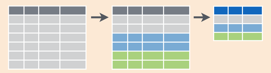
Figure 5.4: Group by and summarize diagram from Data Wrangling with dplyr and tidyr cheatsheet

It’s often more useful to summarize a variable based on the groupings of another variable. Let’s say, we are interested in the mean and standard deviation of temperatures but grouped by month. To be more specific: we want the mean and standard deviation of temperatures

1. split by month.
2. sliced by month.
3. aggregated by month.
4. collapsed over month.

Run the following code:

summary_monthly_temp <- weather %>% 
  group_by(month) %>% 
  summarize(mean = mean(temp, na.rm = TRUE), 
            std_dev = sd(temp, na.rm = TRUE))
summary_monthly_temp

month	mean	std_dev
1	35.63566	10.224635
2	34.27060	6.982378
3	39.88007	6.249278
4	51.74564	8.786168
5	61.79500	9.681644
6	72.18400	7.546371
7	80.06622	7.119898
8	74.46847	5.191615
9	67.37129	8.465902
10	60.07113	8.846035
11	44.99043	10.443805
12	38.44180	9.982432

This code is identical to the previous code that created summary_temp, with an extra group_by(month) added. Grouping the weather dataset by month and then passing this new data frame into summarize yields a data frame that shows the mean and standard deviation of temperature for each month in New York City. Note: Since each row in summary_monthly_temp represents a summary of different rows in weather, the observational units have changed.

It is important to note that group_by doesn’t change the data frame. It sets meta-data (data about the data), specifically the group structure of the data. It is only after we apply the summarize function that the data frame changes.

If we would like to remove this group structure meta-data, we can pipe the resulting data frame into the ungroup() function. For example, say the group structure meta-data is set to be by month via group_by(month), all future summarizations will be reported on a month-by-month basis. If however, we would like to no longer have this and have all summarizations be for all data in a single group (in this case over the entire year of 2013), then pipe the data frame in question through and ungroup() to remove this.

We now revisit the n() counting summary function we introduced in the previous section. For example, suppose we’d like to get a sense for how many flights departed each of the three airports in New York City:

by_origin <- flights %>% 
  group_by(origin) %>% 
  summarize(count = n())
by_origin

origin	count
EWR	120835
JFK	111279
LGA	104662

We see that Newark ("EWR") had the most flights departing in 2013 followed by "JFK" and lastly by LaGuardia ("LGA"). Note there is a subtle but important difference between sum() and n(). While sum() simply adds up a large set of numbers, the latter counts the number of times each of many different values occur.

5.5.1 Grouping by more than one variable

You are not limited to grouping by one variable! Say you wanted to know the number of flights leaving each of the three New York City airports for each month, we can also group by a second variable month: group_by(origin, month).

by_origin_monthly <- flights %>% 
  group_by(origin, month) %>% 
  summarize(count = n())
by_origin_monthly

# A tibble: 36 x 3
# Groups:   origin [3]
   origin month count
   <chr>  <int> <int>
 1 EWR        1  9893
 2 EWR        2  9107
 3 EWR        3 10420
 4 EWR        4 10531
 5 EWR        5 10592
 6 EWR        6 10175
 7 EWR        7 10475
 8 EWR        8 10359
 9 EWR        9  9550
10 EWR       10 10104
# … with 26 more rows

We see there are 36 rows to by_origin_monthly because there are 12 months times 3 airports (EWR, JFK, and LGA). Let’s now pose two questions. First, what if we reverse the order of the grouping i.e. we group_by(month, origin)?

by_monthly_origin <- flights %>% 
  group_by(month, origin) %>% 
  summarize(count = n())
by_monthly_origin

# A tibble: 36 x 3
# Groups:   month [12]
   month origin count
   <int> <chr>  <int>
 1     1 EWR     9893
 2     1 JFK     9161
 3     1 LGA     7950
 4     2 EWR     9107
 5     2 JFK     8421
 6     2 LGA     7423
 7     3 EWR    10420
 8     3 JFK     9697
 9     3 LGA     8717
10     4 EWR    10531
# … with 26 more rows

In by_monthly_origin the month column is now first and the rows are sorted by month instead of origin. If you compare the values of count in by_origin_monthly and by_monthly_origin using the View() function, you’ll see that the values are actually the same, just presented in a different order.

Second, why do we group_by(origin, month) and not group_by(origin) and then group_by(month)? Let’s investigate:

by_origin_monthly_incorrect <- flights %>% 
  group_by(origin) %>% 
  group_by(month) %>% 
  summarize(count = n())
by_origin_monthly_incorrect

# A tibble: 12 x 2
   month count
   <int> <int>
 1     1 27004
 2     2 24951
 3     3 28834
 4     4 28330
 5     5 28796
 6     6 28243
 7     7 29425
 8     8 29327
 9     9 27574
10    10 28889
11    11 27268
12    12 28135

What happened here is that the second group_by(month) overrode the first group_by(origin), so that in the end we are only grouping by month. The lesson here, is if you want to group_by() two or more variables, you should include all these variables in a single group_by() function call.

Learning check

(LC5.5) Recall from Chapter 3 when we looked at plots of temperatures by months in NYC. What does the standard deviation column in the summary_monthly_temp data frame tell us about temperatures in New York City throughout the year?

(LC5.6) What code would be required to get the mean and standard deviation temperature for each day in 2013 for NYC?

(LC5.7) Recreate by_monthly_origin, but instead of grouping via group_by(origin, month), group variables in a different order group_by(month, origin). What differs in the resulting dataset?

(LC5.8) How could we identify how many flights left each of the three airports for each carrier?

(LC5.9) How does the filter operation differ from a group_by followed by a summarize?

5.6 Create new variables/change old variables using mutate

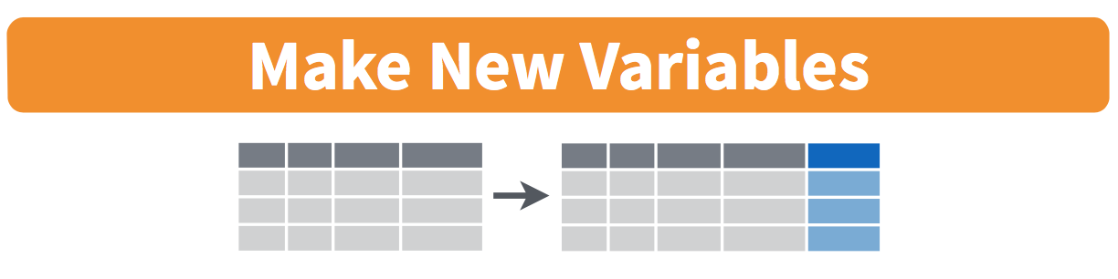
Figure 5.5: Mutate diagram from Data Wrangling with dplyr and tidyr cheatsheet

When looking at the flights dataset, there are some clear additional variables that could be calculated based on the values of variables already in the dataset. Passengers are often frustrated when their flights departs late, but change their mood a bit if pilots can make up some time during the flight to get them to their destination close to when they expected to land. This is commonly referred to as “gain” and we will create this variable using the mutate function. Note that we have also overwritten the flights data frame with what it was before as well as an additional variable gain here, or put differently, the mutate() command outputs a new data frame which then gets saved over the original flights data frame.

flights <- flights %>% 
  mutate(gain = dep_delay - arr_delay)

Let’s take a look at dep_delay, arr_delay, and the resulting gain variables for the first 5 rows in our new flights data frame:

# A tibble: 5 x 3
  dep_delay arr_delay  gain
      <dbl>     <dbl> <dbl>
1         2        11    -9
2         4        20   -16
3         2        33   -31
4        -1       -18    17
5        -6       -25    19

The flight in the first row departed 2 minutes late but arrived 11 minutes late, so its “gained time in the air” is actually a loss of 9 minutes, hence its gain is -9. Contrast this to the flight in the fourth row which departed a minute early (dep_delay of -1) but arrived 18 minutes early (arr_delay of -18), so its “gained time in the air” is 17 minutes, hence its gain is +17.

Why did we overwrite flights instead of assigning the resulting data frame to a new object, like flights_with_gain? As a rough rule of thumb, as long as you are not losing information that you might need later, it’s acceptable practice to overwrite data frames. However, if you overwrite existing variables and/or change the observational units, recovering the original information might prove difficult. In this case, it might make sense to create a new data object.

Let’s look at summary measures of this gain variable and even plot it in the form of a histogram:

gain_summary <- flights %>% 
  summarize(
    min = min(gain, na.rm = TRUE),
    q1 = quantile(gain, 0.25, na.rm = TRUE),
    median = quantile(gain, 0.5, na.rm = TRUE),
    q3 = quantile(gain, 0.75, na.rm = TRUE),
    max = max(gain, na.rm = TRUE),
    mean = mean(gain, na.rm = TRUE),
    sd = sd(gain, na.rm = TRUE),
    missing = sum(is.na(gain))
  )
gain_summary

min	q1	median	q3	max	mean	sd	missing
-196	-3	7	17	109	5.659779	18.04365	9430

We’ve recreated the summary function we saw in Chapter 3 here using the summarize function in dplyr.

ggplot(data = flights, mapping = aes(x = gain)) +
  geom_histogram(color = "white", bins = 20)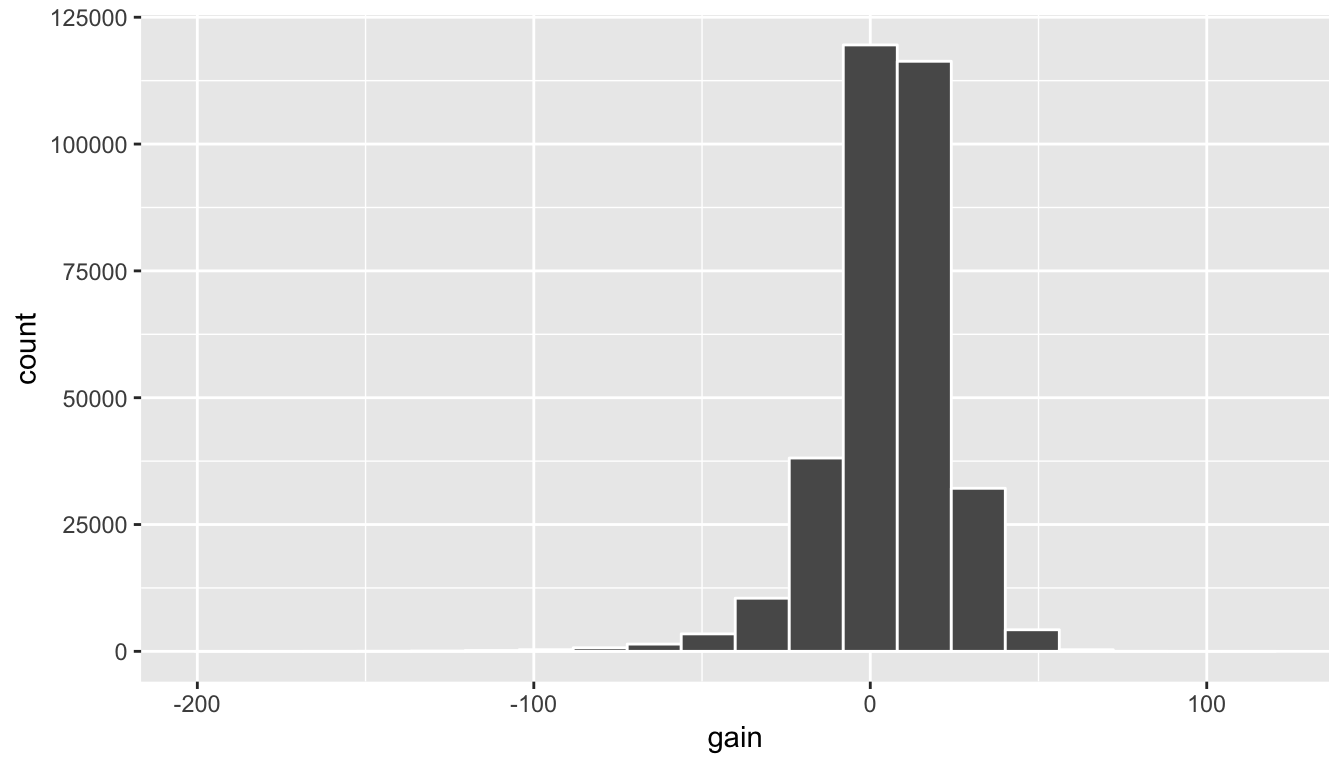

Figure 5.6: Histogram of gain variable

We can also create multiple columns at once and even refer to columns that were just created in a new column. Hadley and Garrett produce one such example in Chapter 5 of “R for Data Science” (Grolemund and Wickham 2016):

flights <- flights %>% 
  mutate(
    gain = dep_delay - arr_delay,
    hours = air_time / 60,
    gain_per_hour = gain / hours
  )

Learning check

(LC5.10) What do positive values of the gain variable in flights correspond to? What about negative values? And what about a zero value?

(LC5.11) Could we create the dep_delay and arr_delay columns by simply subtracting dep_time from sched_dep_time and similarly for arrivals? Try the code out and explain any differences between the result and what actually appears in flights.

(LC5.12) What can we say about the distribution of gain? Describe it in a few sentences using the plot and the gain_summary data frame values.

5.7 Reorder the data frame using arrange

One of the most common things people working with data would like to do is sort the data frames by a specific variable in a column. Have you ever been asked to calculate a median by hand? This requires you to put the data in order from smallest to highest in value. The dplyr package has a function called arrange that we will use to sort/reorder our data according to the values of the specified variable. This is often used after we have used the group_by and summarize functions as we will see.

Let’s suppose we were interested in determining the most frequent destination airports from New York City in 2013:

freq_dest <- flights %>% 
  group_by(dest) %>% 
  summarize(num_flights = n())
freq_dest

# A tibble: 105 x 2
   dest  num_flights
   <chr>       <int>
 1 ABQ           254
 2 ACK           265
 3 ALB           439
 4 ANC             8
 5 ATL         17215
 6 AUS          2439
 7 AVL           275
 8 BDL           443
 9 BGR           375
10 BHM           297
# … with 95 more rows

You’ll see that by default the values of dest are displayed in alphabetical order here. We are interested in finding those airports that appear most:

freq_dest %>% 
  arrange(num_flights)

# A tibble: 105 x 2
   dest  num_flights
   <chr>       <int>
 1 LEX             1
 2 LGA             1
 3 ANC             8
 4 SBN            10
 5 HDN            15
 6 MTJ            15
 7 EYW            17
 8 PSP            19
 9 JAC            25
10 BZN            36
# … with 95 more rows

This is actually giving us the opposite of what we are looking for. It tells us the least frequent destination airports first. To switch the ordering to be descending instead of ascending we use the desc (descending) function:

freq_dest %>% 
  arrange(desc(num_flights))

# A tibble: 105 x 2
   dest  num_flights
   <chr>       <int>
 1 ORD         17283
 2 ATL         17215
 3 LAX         16174
 4 BOS         15508
 5 MCO         14082
 6 CLT         14064
 7 SFO         13331
 8 FLL         12055
 9 MIA         11728
10 DCA          9705
# … with 95 more rows

5.8 Joining data frames

Another common task is joining AKA merging two different datasets. For example, in the flights data, the variable carrier lists the carrier code for the different flights. While "UA" and "AA" might be somewhat easy to guess for some (United and American Airlines), what are “VX”, “HA”, and “B6”? This information is provided in a separate data frame airlines.

View(airlines)

We see that in airports, carrier is the carrier code while name is the full name of the airline. Using this table, we can see that “VX”, “HA”, and “B6” correspond to Virgin America, Hawaiian Airlines, and JetBlue respectively. However, will we have to continually look up the carrier’s name for each flight in the airlines dataset? No! Instead of having to do this manually, we can have R automatically do the “looking up” for us.

Note that the values in the variable carrier in flights match the values in the variable carrier in airlines. In this case, we can use the variable carrier as a key variable to join/merge/match the two data frames by. Key variables are almost always identification variables that uniquely identify the observational units as we saw back in Subsection 4.2.2 on identification vs measurement variables. This ensures that rows in both data frames are appropriate matched during the join. Hadley and Garrett (Grolemund and Wickham 2016) created the following diagram to help us understand how the different datasets are linked by various key variables:

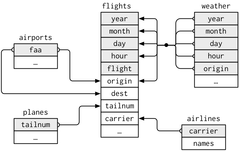
Figure 5.7: Data relationships in nycflights13 from R for Data Science

5.8.1 Joining by “key” variables

In both flights and airlines, the key variable we want to join/merge/match the two data frames with has the same name in both datasets: carriers. We make use of the inner_join() function to join by the variable carrier.

flights_joined <- flights %>% 
  inner_join(airlines, by = "carrier")
View(flights)
View(flights_joined)

We observed that the flights and flights_joined are identical except that flights_joined has an additional variable name whose values were drawn from airlines.

A visual representation of the inner_join is given below (Grolemund and Wickham 2016):

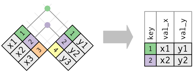
Figure 5.8: Diagram of inner join from R for Data Science

There are more complex joins available, but the inner_join will solve nearly all of the problems you’ll face in our experience.

5.8.2 Joining by “key” variables with different names

Say instead, you are interested in all the destinations of flights from NYC in 2013 and ask yourself:

• “What cities are these airports in?”
• “Is "ORD" Orlando?”
• "Where is "FLL"?

The airports data frame contains airport codes:

View(airports)

However, looking at both the airports and flights and the visual representation of the relations between the data frames in Figure 5.8, we see that in:

• airports the airport code is in the variable faa
• flights the airport code is in the variable origin

So to join these two datasets, our inner_join operation involves a by argument that accounts for the different names:

flights %>% 
  inner_join(airports, by = c("dest" = "faa"))

Let’s construct the sequence of commands that computes the number of flights from NYC to each destination, but also includes information about each destination airport:

named_dests <- flights %>%
  group_by(dest) %>%
  summarize(num_flights = n()) %>%
  arrange(desc(num_flights)) %>%
  inner_join(airports, by = c("dest" = "faa")) %>%
  rename(airport_name = name)
named_dests

# A tibble: 101 x 9
   dest  num_flights airport_name          lat    lon   alt    tz dst   tzone   
   <chr>       <int> <chr>               <dbl>  <dbl> <int> <dbl> <chr> <chr>   
 1 ORD         17283 Chicago Ohare Intl   42.0  -87.9   668    -6 A     America…
 2 ATL         17215 Hartsfield Jackson…  33.6  -84.4  1026    -5 A     America…
 3 LAX         16174 Los Angeles Intl     33.9 -118.    126    -8 A     America…
 4 BOS         15508 General Edward Law…  42.4  -71.0    19    -5 A     America…
 5 MCO         14082 Orlando Intl         28.4  -81.3    96    -5 A     America…
 6 CLT         14064 Charlotte Douglas …  35.2  -80.9   748    -5 A     America…
 7 SFO         13331 San Francisco Intl   37.6 -122.     13    -8 A     America…
 8 FLL         12055 Fort Lauderdale Ho…  26.1  -80.2     9    -5 A     America…
 9 MIA         11728 Miami Intl           25.8  -80.3     8    -5 A     America…
10 DCA          9705 Ronald Reagan Wash…  38.9  -77.0    15    -5 A     America…
# … with 91 more rows

In case you didn’t know, "ORD" is the airport code of Chicago O’Hare airport and "FLL" is the main airport in Fort Lauderdale, Florida, which we can now see in our named_dests data frame.

5.8.3 Joining by multiple “key” variables

Say instead we are in a situation where we need to join by multiple variables. For example, in Figure 5.7 above we see that in order to join the flights and weather data frames, we need more than one key variable: year, month, day, hour, and origin. This is because the combination of these 5 variables act to uniquely identify each observational unit in the weather data frame: hourly weather recordings at each of the 3 NYC airports.

We achieve this by specifying a vector of key variables to join by using the c() concatenate function. Note the individual variables need to be wrapped in quotation marks.

flights_weather_joined <- flights %>%
  inner_join(weather, by = c("year", "month", "day", "hour", "origin"))
flights_weather_joined

# A tibble: 335,220 x 32
    year month   day dep_time sched_dep_time dep_delay arr_time sched_arr_time
   <dbl> <dbl> <int>    <int>          <int>     <dbl>    <int>          <int>
 1  2013     1     1      517            515         2      830            819
 2  2013     1     1      533            529         4      850            830
 3  2013     1     1      542            540         2      923            850
 4  2013     1     1      544            545        -1     1004           1022
 5  2013     1     1      554            600        -6      812            837
 6  2013     1     1      554            558        -4      740            728
 7  2013     1     1      555            600        -5      913            854
 8  2013     1     1      557            600        -3      709            723
 9  2013     1     1      557            600        -3      838            846
10  2013     1     1      558            600        -2      753            745
# … with 335,210 more rows, and 24 more variables: arr_delay <dbl>,
#   carrier <chr>, flight <int>, tailnum <chr>, origin <chr>, dest <chr>,
#   air_time <dbl>, distance <dbl>, hour <dbl>, minute <dbl>,
#   time_hour.x <dttm>, gain <dbl>, hours <dbl>, gain_per_hour <dbl>,
#   temp <dbl>, dewp <dbl>, humid <dbl>, wind_dir <dbl>, wind_speed <dbl>,
#   wind_gust <dbl>, precip <dbl>, pressure <dbl>, visib <dbl>,
#   time_hour.y <dttm>

Learning check

(LC5.13) Looking at Figure 5.7, when joining flights and weather (or, in other words, matching the hourly weather values with each flight), why do we need to join by all of year, month, day, hour, and origin, and not just hour?

(LC5.14) What surprises you about the top 10 destinations from NYC in 2013?

5.9 Other verbs

On top of the following examples of other verbs, if you’d like to see more examples on using dplyr, the data wrangling verbs we introduction in Section 5.2, and the pipe function %>% with the nycflights13 dataset, check out Chapter 5 of Hadley and Garrett’s book (Grolemund and Wickham 2016).

5.9.1 Select variables using select

Figure 5.9: Select diagram from Data Wrangling with dplyr and tidyr cheatsheet

We’ve seen that the flights data frame in the nycflights13 package contains many different variables. The names function gives a listing of all the columns in a data frame; in our case you would run names(flights). You can also identify these variables by running the glimpse function in the dplyr package:

glimpse(flights)

However, say you only want to consider two of these variables, say carrier and flight. You can select these:

flights %>% 
  select(carrier, flight)

This function makes navigating datasets with a very large number of variables easier for humans by restricting consideration to only those of interest, like carrier and flight above. So for example, this might make viewing the dataset using the View() spreadsheet viewer more digestible. However, as far as the computer is concerned it doesn’t care how many variables additional variables are in the dataset in question, so long as carrier and flight are included.

Another example involves the variable year. If you remember the original description of the flights data frame (or by running ?flights), you’ll remember that this data correspond to flights in 2013 departing New York City. The year variable isn’t really a variable here in that it doesn’t vary… flights actually comes from a larger dataset that covers many years. We may want to remove the year variable from our dataset since it won’t be helpful for analysis in this case. We can deselect year by using the - sign:

flights_no_year <- flights %>% 
  select(-year)
names(flights_no_year)

Or we could specify a ranges of columns:

flight_arr_times <- flights %>% 
  select(month:day, arr_time:sched_arr_time)
flight_arr_times

The select function can also be used to reorder columns in combination with the everything helper function. Let’s suppose we’d like the hour, minute, and time_hour variables, which appear at the end of the flights dataset, to actually appear immediately after the day variable:

flights_reorder <- flights %>% 
  select(month:day, hour:time_hour, everything())
names(flights_reorder)

in this case everything() picks up all remaining variables. Lastly, the helper functions starts_with, ends_with, and contains can be used to choose column names that match those conditions:

flights_begin_a <- flights %>% 
  select(starts_with("a"))
flights_begin_a

flights_delays <- flights %>% 
  select(ends_with("delay"))
flights_delays

flights_time <- flights %>% 
  select(contains("time"))
flights_time

5.9.2 Rename variables using rename

Another useful function is rename, which as you may suspect renames one column to another name. Suppose we wanted dep_time and arr_time to be departure_time and arrival_time instead in the flights_time data frame:

flights_time_new <- flights %>% 
  select(contains("time")) %>% 
  rename(departure_time = dep_time,
         arrival_time = arr_time)
names(flights_time)

Note that in this case we used a single = sign with the rename(). Ex: departure_time = dep_time. This is because we are not testing for equality like we would using ==, but instead we want to assign a new variable departure_time to have the same values as dep_time and then delete the variable dep_time.

It’s easy to forget if the new name comes before or after the equals sign. I usually remember this as “New Before, Old After” or NBOA. You’ll receive an error if you try to do it the other way:

Error: Unknown variables: departure_time, arrival_time.

5.9.3 Find the top number of values using top_n

We can also use the top_n function which automatically tells us the most frequent num_flights. We specify the top 10 airports here:

named_dests %>% 
  top_n(n = 10, wt = num_flights)

We’ll still need to arrange this by num_flights though:

named_dests  %>% 
  top_n(n = 10, wt = num_flights) %>% 
  arrange(desc(num_flights))

Note: Remember that I didn’t pull the n and wt arguments out of thin air. They can be found by using the ? function on top_n.

We can go one stop further and tie together the group_by and summarize functions we used to find the most frequent flights:

ten_freq_dests <- flights %>%
  group_by(dest) %>%
  summarize(num_flights = n()) %>%
  arrange(desc(num_flights)) %>%
  top_n(n = 10) 
View(ten_freq_dests)

Learning check

(LC5.15) What are some ways to select all three of the dest, air_time, and distance variables from flights? Give the code showing how to do this in at least three different ways.

(LC5.16) How could one use starts_with, ends_with, and contains to select columns from the flights data frame? Provide three different examples in total: one for starts_with, one for ends_with, and one for contains.

(LC5.17) Why might we want to use the select function on a data frame?

(LC5.18) Create a new data frame that shows the top 5 airports with the largest arrival delays from NYC in 2013.

5.10 Conclusion

5.10.1 Putting it all together: Available seat miles

Let’s recap a selection of verbs in Table 5.1 summarizing their differences. Using these verbs and the pipe %>% operator from Section 5.1, you’ll be able to write easily legible code to perform almost all the data wrangling necessary for the rest of this book.

Table 5.1: Summary of data wrangling verbs

	Verb	Data wrangling operation
1	filter()	Pick out a subset of rows
2	summarize()	Summarize many values to one using a summary statistic function like mean(), median(), etc.
3	group_by()	Add grouping structure to rows in data frame. Note this does not change values in data frame.
4	mutate()	Create new variables by mutating existing ones
5	arrange()	Arrange rows of a data variable in ascending (default) or descending order
6	inner_join()	Join/merge two data frames, matching rows by a key variable
7	select()	Pick out a subset of columns to make data frames easier to view

Let’s now put your newly acquired data wrangling skills to the test! An airline industry measure of a passenger airline’s capacity is the available seat miles, which is equal to the number of seats available multiplied by the number of miles or kilometers flown. So for example say an airline had 2 flights using a plane with 10 seats that flew 500 miles and 3 flights using a plane with 20 seats that flew 1000 miles, the available seat miles would be 2 \(\times\) 10 \(\times\) 500 \(+\) 3 \(\times\) 20 \(\times\) 1000 = 70,000 seat miles.

Learning check

(LC5.19) Using the datasets included in the nycflights13 package, compute the available seat miles for each airline sorted in descending order. After completing all the necessary data wrangling steps, the resulting data frame should have 16 rows (one for each airline) and 2 columns (airline name and available seat miles). Here are some hints:

1. Crucial: Unless you are very confident in what you are doing, it is worthwhile to not starting coding right away, but rather first sketch out on paper all the necessary data wrangling steps not using exact code, but rather high-level pseudocode that is informal yet detailed enough to articulate what you are doing. This way you won’t confuse what you are trying to do (the algorithm) with how you are going to do it (writing dplyr code).
2. Take a close look at all the datasets using the View() function: flights, weather, planes, airports, and airlines to identify which variables are necessary to compute available seat miles.
3. Figure 5.7 above showing how the various datasets can be joined will also be useful.
4. Consider the data wrangling verbs in Table 5.1 as your toolbox!

5.10.2 Review questions

Review questions have been designed using the fivethirtyeight R package (Kim, Ismay, and Chunn 2019) with links to the corresponding FiveThirtyEight.com articles in our free DataCamp course Effective Data Storytelling using the tidyverse. The material in this chapter is covered in the chapters of the DataCamp course available below:

• Filtering, Grouping, & Summarizing
• dplyr Review

5.10.3 What’s to come?

Congratulations! We’ve completed the “data science” portion of this book! We’ll now move to the “data modeling” portion in Chapters 6 and 7, where you’ll leverage your data visualization and wrangling skills to model the relationships between different variables of datasets. However, we’re going to leave “Inference for Regression” (Chapter 11) until later.

5.10.4 Resources

As we saw with the RStudio cheatsheet on data visualization, RStudio has also created a cheatsheet for data wrangling entitled “Data Transformation with dplyr”.

5.10.5 Script of R code

An R script file of all R code used in this chapter is available here.