11 Inference for Regression

---

Note: This chapter is still under construction. If you would like to contribute, please check us out on GitHub at https://github.com/moderndive/moderndive_book.

---

11.1 Refresher: Professor evaluations data

Let’s revisit the professor evaluations data that we analyzed using multiple regression with one numerical and one categorical predictor. In particular

• \(y\): outcome variable of instructor evaluation score
• predictor variables
  • \(x_1\): numerical explanatory/predictor variable of age
  • \(x_2\): categorical explanatory/predictor variable of gender

library(ggplot2)
library(dplyr)
library(moderndive)

load(url("http://www.openintro.org/stat/data/evals.RData"))
evals <- evals %>%
  select(score, ethnicity, gender, language, age, bty_avg, rank)

First, recall that we had two competing potential models to explain professors’ teaching scores:

1. Model 1: No interaction term. i.e. both male and female profs have the same slope describing the associated effect of age on teaching score
2. Model 2: Includes an interaction term. i.e. we allow for male and female profs to have different slopes describing the associated effect of age on teaching score

11.1.1 Refresher: Visualizations

Recall the plots we made for both these models:

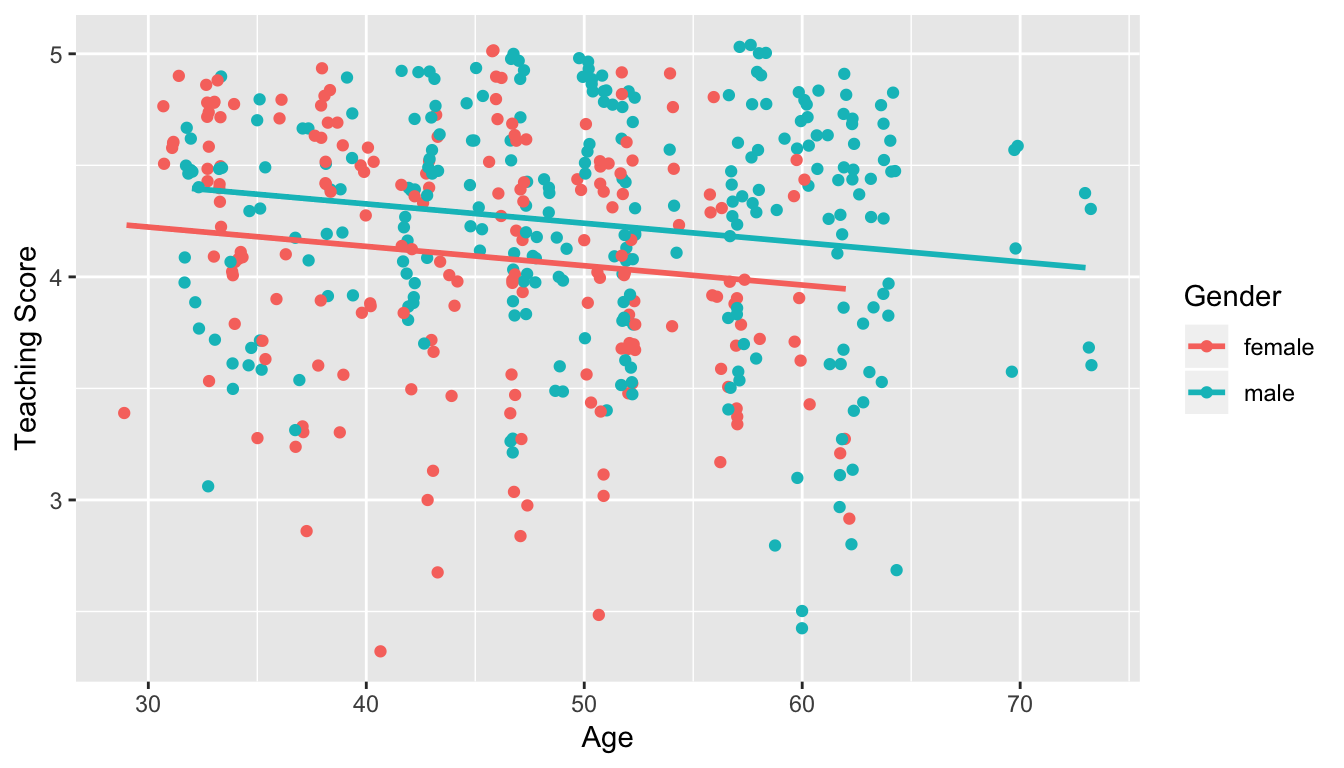
Figure 11.1: Model 1: no interaction effect included

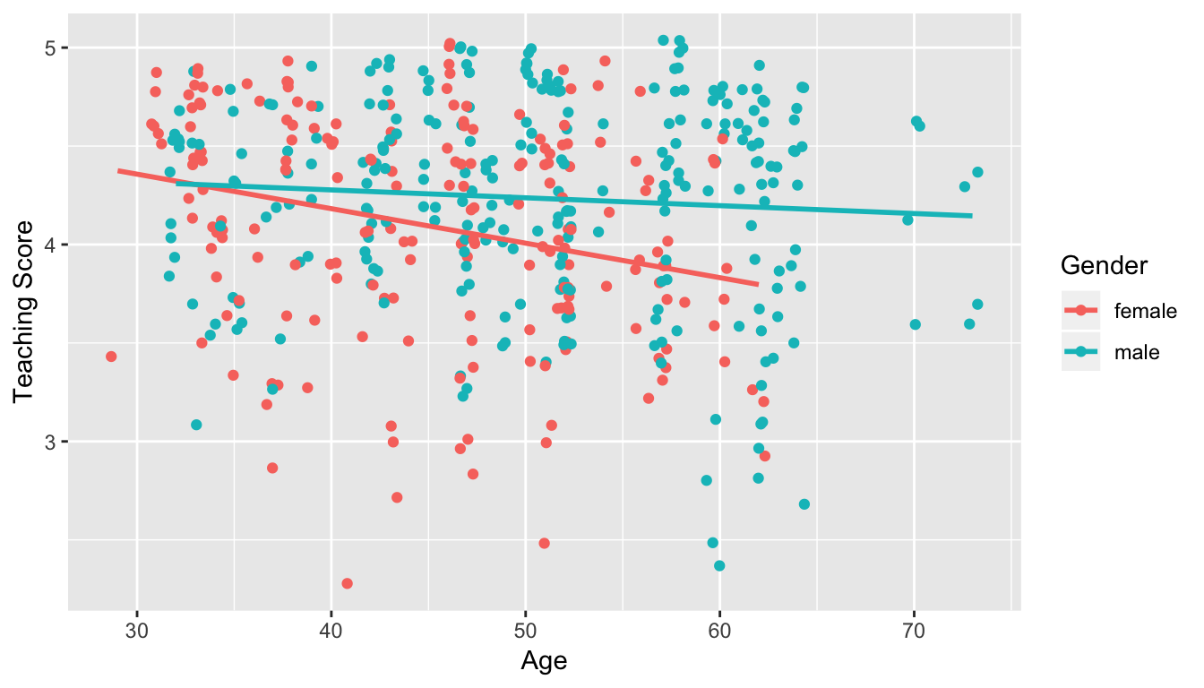
Figure 11.2: Model 2: interaction effect included

11.1.2 Refresher: Regression tables

Last, let’s recall the regressions we fit. First, the regression with no interaction effect: note the use of + in the formula.

score_model_2 <- lm(score ~ age + gender, data = evals)
get_regression_table(score_model_2)

Table 11.1: Model 1: Regression table with no interaction effect included

term	estimate	std_error	statistic	p_value	lower_ci	upper_ci
intercept	4.484	0.125	35.79	0.000	4.238	4.730
age	-0.009	0.003	-3.28	0.001	-0.014	-0.003
gendermale	0.191	0.052	3.63	0.000	0.087	0.294

Second, the regression with an interaction effect: note the use of * in the formula.

score_model_3 <- lm(score ~ age * gender, data = evals)
get_regression_table(score_model_3)

Table 11.2: Model 2: Regression table with interaction effect included

term	estimate	std_error	statistic	p_value	lower_ci	upper_ci
intercept	4.883	0.205	23.80	0.000	4.480	5.286
age	-0.018	0.004	-3.92	0.000	-0.026	-0.009
gendermale	-0.446	0.265	-1.68	0.094	-0.968	0.076
age:gendermale	0.014	0.006	2.45	0.015	0.003	0.024

11.1.3 Script of R code

An R script file of all R code used in this chapter is available here.