Mapping the show

library(steves)
library(dplyr)
#> 
#> Attaching package: 'dplyr'
#> The following objects are masked from 'package:stats':
#> 
#>     filter, lag
#> The following objects are masked from 'package:base':
#> 
#>     intersect, setdiff, setequal, union
library(ggplot2)

Where does the show go?

primary_destination is geocoded to lat / long via OSM Nominatim, with a fallback chain (full place → first place name → country centroid → average of capital cities for multi-country compilations). The geo_match column flags which tier resolved each row, so you can filter out coarse fallbacks for sharper maps.

episodes |>
  count(geo_match)
#> # A tibble: 5 × 2
#>   geo_match     n
#>   <chr>     <int>
#> 1 centroid      9
#> 2 country       8
#> 3 full        108
#> 4 simple       23
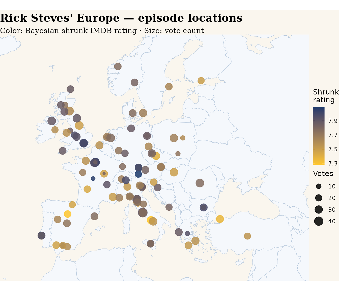
#> 5 NA           11

A static atlas

world <- map_data("world")

episodes |>
  filter(!is.na(lat), geo_match %in% c("full", "simple")) |>
  ggplot() +
  geom_polygon(data = world,
               aes(long, lat, group = group),
               fill = "#F5F8FC", color = "#B5C7DB", linewidth = 0.2) +
  geom_point(aes(long, lat, color = imdb_rating_shrunk,
                 size = imdb_votes),
             alpha = 0.85) +
  coord_quickmap(xlim = c(-15, 45), ylim = c(34, 65)) +
  scale_color_gradient(low = "#FFC72C", high = "#1B3A6B",
                       name = "Shrunk\nrating") +
  scale_size_continuous(range = c(1.5, 6), name = "Votes") +
  labs(title = "Rick Steves' Europe — episode locations",
       subtitle = "Color: Bayesian-shrunk IMDB rating · Size: vote count",
       x = NULL, y = NULL) +
  theme_void() +
  theme(plot.background  = element_rect(fill = "#FAF6EE", color = NA),
        panel.background = element_rect(fill = "#FAF6EE", color = NA),
        plot.title       = element_text(family = "serif",
                                        face = "bold", size = 16),
        plot.subtitle    = element_text(family = "serif", size = 11))
#> Warning: Removed 7 rows containing missing values or values outside the scale range
#> (`geom_point()`).

Country revisits

A few cities (Paris, Rome, Venice) get multiple episodes over the years. Easy to find:

episodes |>
  count(primary_destination, sort = TRUE) |>
  filter(n > 1) |>
  head(10)
#> # A tibble: 10 × 2
#>    primary_destination     n
#>    <chr>               <int>
#>  1 Various                17
#>  2 Rome                    6
#>  3 London                  5
#>  4 Paris                   5
#>  5 Florence                3
#>  6 Istanbul                3
#>  7 Sicily                  3
#>  8 Amsterdam               2
#>  9 Berlin                  2
#> 10 Bulgaria                2